Example usage of create_risk_report(), applied to create reports for French Viticultural areas
Samuel M. Owens1
2025-08-07
Source:vignettes/150_create_risk_report_example_usage.Rmd
150_create_risk_report_example_usage.RmdOverview
In the last few vignettes, I have created various outputs that help me to analyze the risk of SLF establishment at for global viticultural regions. I created risk maps and tables, range shift maps and tables, risk quadrant maps for viticultural regions and SLF populations, and have calculated various summary statistics such as omission and commission error, area under the curve, and the optimal suitability threshold for each model.
In this vignette, I will use my function
create_risk_report() to refine each of these outputs
(excluding the summary statistics, which area model-specific) for
countries and provinces of key importance for global viticulture. These
outputs will crop maps and viticultural region risk assessments for each
region of interest. I will begin by creating a report for each country
in our input the wineries_esri54017_tidied dataset. I will
also create reports for key areas where viticulture is expected to
expand or decline under climate change. This vignette will also outline
the best practice for usage of my function
create_risk_report().
Setup
# general tools
library(tidyverse)
library(cli)
library(here)
library(common)

# spatial data
library(terra)
library(sf)
library(rnaturalearth)
library(rnaturalearthhires)
library(rnaturalearthdata)
library(ggspatial)

# aesthetics
library(kableExtra)
library(formattable)
library(webshot)
library(webshot2)
library(ggnewscale) ## MUST use version 0.4.10- 0.5.0 has a bug that breaks this function

# for analysis
library(patchwork)
library(gginnards)

library(scari)
Create internal dataset for function
You should only need to do this once, and again each time you change the input data.
I will start by creating an internal dataset to be used by the
function. These datasets were created in the previous vignettes and are
stored in the data or data-raw folders of the
package. I will import these datasets and save them as internal datasets
for the function to use.
If you have other datasets to use, you can replace the datasets below with your own, so long as they are in a similar format.
# .csv files
threshold_exponential_values <- read.csv(file = file.path(here::here(), "data-raw", "threshold_exponential_values.csv"))
# .rds files
IVR_locations <- readr::read_rds(file = file.path(here::here(), "data", "wineries_esri54017_tidied.rds"))
summary_global <- readr::read_rds(file = file.path(here::here(), "data", "global_threshold_values.rds"))
summary_regional_ensemble <- readr::read_rds(file = file.path(here::here(), "data", "ensemble_threshold_values.rds"))
# predicted xy suitability
xy_global_hist <- readr::read_rds(file = file.path(here::here(), "data", "global_wineries_1981-2010_xy_pred_suit.rds"))
xy_global_future <- readr::read_rds(file = file.path(here::here(), "data", "global_wineries_2041-2070_GFDL_ssp_mean_xy_pred_suit.rds"))
xy_regional_ensemble_hist <- readr::read_rds(file = file.path(here::here(), "data", "regional_ensemble_wineries_1981-2010_xy_pred_suit.rds"))
xy_regional_ensemble_future <- readr::read_rds(file = file.path(here::here(), "data", "regional_ensemble_wineries_2041-2070_GFDL_ssp_mean_xy_pred_suit.rds"))
I need to make some edits to the xy datasets.
xy_global_hist <- dplyr::rename(xy_global_hist, "xy_global_hist" = "xy_global_1995")
xy_global_future <- dplyr::rename(xy_global_future, "xy_global_future" = "xy_global_2055")
xy_regional_ensemble_hist <- dplyr::rename(xy_regional_ensemble_hist, "xy_regional_ensemble_hist" = "xy_regional_ensemble_1995")
xy_regional_ensemble_future <- dplyr::rename(xy_regional_ensemble_future, "xy_regional_ensemble_future" = "xy_regional_ensemble_2055")
# mypath
mypath <- file.path(here::here() %>%
                       dirname(),
                     "maxent/models")

# import raster files
## historical raster
slf_binarized_hist <- terra::rast(x = file.path(mypath, "working_dir", "slf_binarized_summed_1981-2010.asc"))
slf_binarized_future <- terra::rast(x = file.path(mypath, "working_dir", "slf_binarized_summed_2041-2070_ssp_mean_GFDL.asc"))
slf_range_shift <- terra::rast(x = file.path(mypath, "working_dir", "slf_range_shift_summed_ssp_mean_GFDL.asc"))

# write to proper folder
terra::writeRaster(
  slf_binarized_hist,
  filename = file.path(here::here(), "vignette-outputs", "rasters", "slf_binarized_summed_1981-2010.asc"),
  overwrite = FALSE
)

terra::writeRaster(
  slf_binarized_future,
  filename = file.path(here::here(), "vignette-outputs", "rasters", "slf_binarized_summed_2041-2070_ssp_mean_GFDL.asc"),
  overwrite = FALSE
)

terra::writeRaster(
  slf_range_shift,
  filename = file.path(here::here(), "vignette-outputs", "rasters", "slf_range_shift_summed_ssp_mean_GFDL.asc"),
  overwrite = FALSE
)
# transform all data frames to internal dataset
usethis::use_data(
  threshold_exponential_values, IVR_locations, summary_global, summary_regional_ensemble, xy_global_hist, xy_global_future, xy_regional_ensemble_hist, xy_regional_ensemble_future,
  internal = TRUE,
  overwrite = FALSE
)
The internal dataset sysdata.rda is used for this
function in the remainder of the vignette; this file is stored at
root/R.
Example usage for create_risk_report(): France
I will now pull out a specific example of France to analyze and demonstrate usage of this function. I will use France as a case study. Here is an example of the code we could use to retrieve a report for France. We will work through each argument:
scari::create_risk_report(
  locality.iso = "fra", # A3-iso
  locality.name = "France", #name
  locality.type = "country", # record type
  # saving output
  mypath = file.path(here::here(), "vignette-outputs", "reports", "France"), # the output location
  create.dir = FALSE, # not saving so not necessary
  save.report = FALSE, # dont save, this is an example
  raster.path = file.path(here::here(), "vignette-outputs", "rasters"), # path to rasters
  # aesthetics- dont necessarily need to be specified
  buffer.dist = 20000, # 20km, this is the distance at which buffers should be drawn on maps to indicate IVR suitability predictions
  period.present = "1981-2010",
  period.projected = "2041-2070",
  model.projected = "GFDL-ESM4",
  ssp.projected = "ssp_126_370_585",
  crs = "ESRI:54017"
)
First, we need to look up the A3-iso code for France. It is “FRA”. We also need to specify that this is a country.
Now, we need to specify arguments for the report output.
mypath specifies the path to the directory where this will
be saved. It is not necessary if the report will not be saved (ie,
create.dir = FALSE and save.report = FALSE).
The argument raster.path specifies where the rasters are
stored for this function. They are pre-loaded above and by default are
stored in root/vignette-outputs/rasters.
Next, we can optionally specify arguments for the aesthetics. If not specified, they will default to a specified value. I have listed the defaults in the example. Note that if you change any of these from their defaults, you should ensure that you have first changed the input datasets, which I created above. This would require you to rerun the package vignettes. I will give an explanation and list out the arguments below:
buffer.dist: this specifies the distance at which a
buffer is drawn around important viticultural regions (IVRs) to
calculate the suitability. The max suitability is taken from this buffer
region. If left blank, it will assume that you instead used a simple
point-wise calculation of suitability (aka, the suitability was taken at
the exact point locations of IVRs). NOTE: if you choose to
change this here, it will only change the aesthetic and not the
calculations (the data are created in vignette 130 and pre-loaded
above.) You should change the buffer distance used in that vignette if
you wish to make this change.
period.present: The time period of the historical
data.
period.projected: The time period for the projected
future data.
model.projected: The model used for the projected future
data.
ssp.projected: The shared socioeconomic pathway (SSP)
used for the projected future data. This is a scenario of future climate
change that is used to project future conditions.
crs: The crs chosen for all input data and rasters. Note
that changing this would require a complete rerun of the package
vignettes.
Finally, we have map.style, which is a purely aesthetic
argument. It should be specified as a list argument if not the default
(the default is shown below). Again, this does not need to be
specified.
  # map stype argument as a list
  map.style <- list(
      xlab("UTM_eastings"), # if raster is in lonlat, label as lon/lat, otherwise UTM
      ylab("UTM_northings"), # if raster is in lonlat, label as lon/lat, otherwise UTM
      # aesthetics
      theme_classic(),
      theme(
        # legend
        legend.position = "bottom",
        legend.key = element_rect(color = "black")
      ),
      guides(fill = guide_legend(nrow = 1, byrow = TRUE)),
      # scales
      scale_x_continuous(expand = c(0, 0)),
      scale_y_continuous(expand = c(0, 0))
    )
Now, lets call the various elements of this report.
First, we have the summary of this report, which shows important data.
france_slf_risk_report[["Report_info"]]## # A tibble: 6 × 2
## Report_info value
## <chr> <chr>
## 1 Report prepared for: France
## 2 Locality Type: Country
## 3 Time period of present risk based on historical data: 1981-2010
## 4 Time period of future risk projection: 2041-2070
## 5 CMIP6 model used for future risk projection: GFDL-ESM4
## 6 SSP scenarios included: ssp_126_370_585Next, we have a summary of the viticultural regions in France, which shows each IVR (winery), its published coordinates, and the risk associated with each winery:
france_slf_risk_report[["viticultural_regions_list"]]| ID | x | y | Continent | Country | Region | Sub-Region | global_model_risk_present | global_model_risk_future | regional_ensemble_model_risk_present | regional_ensemble_model_risk_future | risk_level_present | risk_count_present | risk_level_future | risk_count_future | risk_shift | risk_shift_count |
|---|---|---|---|---|---|---|---|---|---|---|---|---|---|---|---|---|
| 400 | 723647.102 | 5488176 | Europe | france | alsace__alsace_wine | NA | 10.00 | 10.00 | 9.60 | 9.16 | extreme | 4 | extreme | 4 | extreme-extreme | 0 |
| 401 | -32939.344 | 5137501 | Europe | france | bordeaux__bordeaux_wine | Barsac | 3.43 | 0.10 | 8.09 | 5.12 | high | 3 | high | 3 | high-high | 0 |
| 402 | -51406.925 | 5166040 | Europe | france | bordeaux__bordeaux_wine | Entre-Deux-Mers | 0.54 | 0.21 | 7.97 | 4.68 | high | 3 | low | 1 | high-low | -2 |
| 403 | -26238.908 | 5173287 | Europe | france | bordeaux__bordeaux_wine | Fronsac | 0.85 | 0.27 | 8.05 | 5.65 | high | 3 | high | 3 | high-high | 0 |
| 404 | -29228.589 | 5169499 | Europe | france | bordeaux__bordeaux_wine | Graves | 0.65 | 0.22 | 8.05 | 5.08 | high | 3 | high | 3 | high-high | 0 |
| 405 | -59574.392 | 5178231 | Europe | france | bordeaux__bordeaux_wine | Haut-Médoc | 0.38 | 0.21 | 7.91 | 4.49 | high | 3 | low | 1 | high-low | -2 |
| 406 | -65181.843 | 5183910 | Europe | france | bordeaux__bordeaux_wine | Margaux | 0.38 | 0.19 | 7.91 | 4.45 | high | 3 | low | 1 | high-low | -2 |
| 407 | -96486.280 | 5180102 | Europe | france | bordeaux__bordeaux_wine | Médoc | 0.21 | 0.11 | 7.63 | 4.14 | high | 3 | low | 1 | high-low | -2 |
| 408 | -72257.503 | 5198234 | Europe | france | bordeaux__bordeaux_wine | Pauillac | 0.19 | 0.16 | 7.84 | 4.40 | high | 3 | low | 1 | high-low | -2 |
| 409 | -59117.819 | 5154778 | Europe | france | bordeaux__bordeaux_wine | Pessac-Léognan | 2.35 | 0.34 | 7.91 | 4.66 | high | 3 | low | 1 | high-low | -2 |
| 410 | -19216.851 | 5173994 | Europe | france | bordeaux__bordeaux_wine | Pomerol | 0.85 | 0.27 | 8.09 | 5.65 | high | 3 | high | 3 | high-high | 0 |
| 411 | -16003.697 | 5170869 | Europe | france | bordeaux__bordeaux_wine | Saint-Émilion | 1.59 | 0.21 | 8.13 | 5.36 | high | 3 | high | 3 | high-high | 0 |
| 412 | -74288.743 | 5202759 | Europe | france | bordeaux__bordeaux_wine | Saint-Estèphe | 0.18 | 0.10 | 7.82 | 4.37 | high | 3 | low | 1 | high-low | -2 |
| 413 | -71687.377 | 5194119 | Europe | france | bordeaux__bordeaux_wine | Saint-Julien | 0.19 | 0.16 | 7.84 | 4.40 | high | 3 | low | 1 | high-low | -2 |
| 414 | -31715.040 | 5138593 | Europe | france | bordeaux__bordeaux_wine | Sauternes – Sauternes | 3.43 | 0.10 | 8.09 | 5.12 | high | 3 | high | 3 | high-high | 0 |
| 415 | 448661.203 | 5283498 | Europe | france | burgundy_(bourgogne)__burgundy_wine | Beaujolais | 10.00 | 10.00 | 9.55 | 9.08 | extreme | 4 | extreme | 4 | extreme-extreme | 0 |
| 416 | 541963.436 | 5262718 | Europe | france | burgundy_(bourgogne)__burgundy_wine | Bugey | 10.00 | 10.00 | 9.47 | 8.96 | extreme | 4 | extreme | 4 | extreme-extreme | 0 |
| 417 | 366406.649 | 5429494 | Europe | france | burgundy_(bourgogne)__burgundy_wine | Chablis | 8.74 | 8.27 | 9.35 | 8.67 | extreme | 4 | extreme | 4 | extreme-extreme | 0 |
| 418 | 453485.517 | 5341888 | Europe | france | burgundy_(bourgogne)__burgundy_wine | Côte Chalonnaise | 9.60 | 9.42 | 9.32 | 8.58 | extreme | 4 | extreme | 4 | extreme-extreme | 0 |
| 419 | 466350.355 | 5394939 | Europe | france | burgundy_(bourgogne)__burgundy_wine | Côte d’Or | 10.00 | 10.00 | 9.33 | 9.01 | extreme | 4 | extreme | 4 | extreme-extreme | 0 |
| 420 | 461204.420 | 5357691 | Europe | france | burgundy_(bourgogne)__burgundy_wine | Côte de Beaune | 9.96 | 9.04 | 9.32 | 8.90 | extreme | 4 | extreme | 4 | extreme-extreme | 0 |
| 421 | 468950.124 | 5364381 | Europe | france | burgundy_(bourgogne)__burgundy_wine | Aloxe-Corton | 9.96 | 9.04 | 9.32 | 8.84 | extreme | 4 | extreme | 4 | extreme-extreme | 0 |
| 422 | 458202.624 | 5357472 | Europe | france | burgundy_(bourgogne)__burgundy_wine | Auxey-Duresses | 9.96 | 9.04 | 9.32 | 8.90 | extreme | 4 | extreme | 4 | extreme-extreme | 0 |
| 423 | 466966.795 | 5360757 | Europe | france | burgundy_(bourgogne)__burgundy_wine | Beaune | 9.96 | 9.04 | 9.32 | 8.84 | extreme | 4 | extreme | 4 | extreme-extreme | 0 |
| 424 | 456299.700 | 5353111 | Europe | france | burgundy_(bourgogne)__burgundy_wine | Chassagne-Montrachet | 9.96 | 9.04 | 9.32 | 8.76 | extreme | 4 | extreme | 4 | extreme-extreme | 0 |
| 425 | 460346.764 | 5356717 | Europe | france | burgundy_(bourgogne)__burgundy_wine | Meursault | 9.96 | 9.04 | 9.32 | 8.90 | extreme | 4 | extreme | 4 | extreme-extreme | 0 |
| 426 | 453297.905 | 5350991 | Europe | france | burgundy_(bourgogne)__burgundy_wine | Santenay | 9.96 | 8.01 | 9.32 | 8.76 | extreme | 4 | extreme | 4 | extreme-extreme | 0 |
| 427 | 478571.950 | 5374314 | Europe | france | burgundy_(bourgogne)__burgundy_wine | Côte de Nuits | 9.92 | 9.04 | 9.32 | 8.84 | extreme | 4 | extreme | 4 | extreme-extreme | 0 |
| 428 | 477928.708 | 5374872 | Europe | france | burgundy_(bourgogne)__burgundy_wine | Chambolle-Musigny | 10.00 | 9.57 | 9.32 | 8.96 | extreme | 4 | extreme | 4 | extreme-extreme | 0 |
| 429 | 479349.201 | 5378437 | Europe | france | burgundy_(bourgogne)__burgundy_wine | Gevrey-Chambertin | 10.00 | 9.57 | 9.32 | 8.96 | extreme | 4 | extreme | 4 | extreme-extreme | 0 |
| 430 | 477714.294 | 5370674 | Europe | france | burgundy_(bourgogne)__burgundy_wine | Nuits-Saint-Georges | 9.92 | 9.04 | 9.32 | 8.84 | extreme | 4 | extreme | 4 | extreme-extreme | 0 |
| 431 | 478035.915 | 5372592 | Europe | france | burgundy_(bourgogne)__burgundy_wine | Vosne-Romanée | 9.92 | 9.04 | 9.32 | 8.84 | extreme | 4 | extreme | 4 | extreme-extreme | 0 |
| 432 | 457344.968 | 5300379 | Europe | france | burgundy_(bourgogne)__burgundy_wine | Mâconnais | 10.00 | 10.00 | 9.54 | 9.02 | extreme | 4 | extreme | 4 | extreme-extreme | 0 |
| 433 | 457351.144 | 5295863 | Europe | france | burgundy_(bourgogne)__burgundy_wine | Pouilly-Fuissé | 10.00 | 10.00 | 9.54 | 9.02 | extreme | 4 | extreme | 4 | extreme-extreme | 0 |
| 434 | 385945.121 | 5530554 | Europe | france | champagne__champagne | NA | 9.80 | 9.39 | 9.35 | 8.93 | extreme | 4 | extreme | 4 | extreme-extreme | 0 |
| 435 | 535927.683 | 5330026 | Europe | france | jura__jura_wine | NA | 10.00 | 9.95 | 9.21 | 8.92 | extreme | 4 | extreme | 4 | extreme-extreme | 0 |
| 436 | 301814.874 | 4946650 | Europe | france | languedoc_roussillon | Banyuls | 0.46 | 0.47 | 7.60 | 6.54 | high | 3 | high | 3 | high-high | 0 |
| 437 | 214119.137 | 5000805 | Europe | france | languedoc_roussillon | Blanquette de Limoux | 2.75 | 4.34 | 8.65 | 8.19 | high | 3 | high | 3 | high-high | 0 |
| 438 | 219381.627 | 5032602 | Europe | france | languedoc_roussillon | Cabardès | 3.85 | 3.45 | 8.65 | 8.19 | high | 3 | high | 3 | high-high | 0 |
| 439 | 297311.752 | 4950776 | Europe | france | languedoc_roussillon | Collioure | 0.46 | 0.47 | 7.60 | 6.54 | high | 3 | high | 3 | high-high | 0 |
| 440 | 472241.099 | 5188361 | Europe | france | languedoc_roussillon | Corbières | 7.56 | 5.12 | 8.17 | 7.92 | extreme | 4 | extreme | 4 | extreme-extreme | 0 |
| 441 | 279381.385 | 4982721 | Europe | france | languedoc_roussillon | Côtes du Roussillon | 0.35 | 0.26 | 7.54 | 5.40 | high | 3 | high | 3 | high-high | 0 |
| 442 | 287475.512 | 4985465 | Europe | france | languedoc_roussillon | Fitou | 0.33 | 0.14 | 7.43 | 5.28 | high | 3 | high | 3 | high-high | 0 |
| 443 | 250355.095 | 4977727 | Europe | france | languedoc_roussillon | Maury | 0.54 | 0.62 | 7.97 | 7.59 | high | 3 | high | 3 | high-high | 0 |
| 444 | 243038.616 | 5026028 | Europe | france | languedoc_roussillon | Minervois | 3.89 | 3.99 | 8.16 | 7.81 | high | 3 | high | 3 | high-high | 0 |
| 445 | 277369.110 | 4973722 | Europe | france | languedoc_roussillon | Rivesaltes | 0.35 | 0.26 | 7.62 | 5.35 | high | 3 | high | 3 | high-high | 0 |
| 446 | 471314.734 | 5211713 | Europe | france | loire_valley_loire_valley(wine_region) | Anjou – Saumur | 7.56 | 5.03 | 8.33 | 8.10 | extreme | 4 | extreme | 4 | extreme-extreme | 0 |
| 447 | -32162.093 | 5243288 | Europe | france | loire_valley_loire_valley(wine_region) | Cognac | 0.39 | 0.54 | 7.99 | 6.31 | high | 3 | high | 3 | high-high | 0 |
| 448 | -134993.955 | 5371562 | Europe | france | loire_valley_loire_valley(wine_region) | Muscadet | 0.23 | 0.26 | 7.82 | 7.13 | high | 3 | high | 3 | high-high | 0 |
| 449 | 342207.697 | 5369452 | Europe | france | loire_valley_loire_valley(wine_region) | Pouilly-Fumé | 10.00 | 9.99 | 9.59 | 8.89 | extreme | 4 | extreme | 4 | extreme-extreme | 0 |
| 450 | 274021.036 | 5387566 | Europe | france | loire_valley_loire_valley(wine_region) | Sancerre | 9.65 | 8.92 | 9.32 | 8.43 | extreme | 4 | extreme | 4 | extreme-extreme | 0 |
| 451 | 65900.129 | 5393490 | Europe | france | loire_valley_loire_valley(wine_region) | Touraine | 2.27 | 0.48 | 8.52 | 7.96 | high | 3 | high | 3 | high-high | 0 |
| 452 | 578917.682 | 5530554 | Europe | france | lorraine | NA | 10.00 | 9.09 | 9.33 | 8.81 | extreme | 4 | extreme | 4 | extreme-extreme | 0 |
| 453 | -5574.763 | 5046740 | Europe | france | madiran | NA | 7.32 | 2.16 | 8.66 | 6.76 | extreme | 4 | high | 3 | extreme-high | -1 |
| 454 | 530674.541 | 5042137 | Europe | france | provence | NA | 1.79 | 0.85 | 7.94 | 7.68 | high | 3 | high | 3 | high-high | 0 |
| 455 | 485433.197 | 5099916 | Europe | france | rhône__rhône_wine | Beaumes-de-Venise | 8.72 | 8.56 | 7.86 | 7.75 | extreme | 4 | extreme | 4 | extreme-extreme | 0 |
| 456 | 458476.945 | 5220820 | Europe | france | rhône__rhône_wine | Château-Grillet | 9.12 | 4.19 | 8.22 | 8.03 | extreme | 4 | high | 3 | extreme-high | -1 |
| 457 | 466212.058 | 5093763 | Europe | france | rhône__rhône_wine | Châteauneuf-du-Pape | 0.47 | 0.51 | 7.90 | 5.37 | high | 3 | high | 3 | high-high | 0 |
| 458 | 460078.746 | 5222062 | Europe | france | rhône__rhône_wine | Condrieu | 9.12 | 4.19 | 8.22 | 8.03 | extreme | 4 | high | 3 | extreme-high | -1 |
| 459 | 467958.459 | 5176569 | Europe | france | rhône__rhône_wine | Cornas | 8.83 | 5.85 | 8.03 | 7.78 | extreme | 4 | extreme | 4 | extreme-extreme | 0 |
| 460 | 466937.055 | 5187203 | Europe | france | rhône__rhône_wine | Côte du Rhône-Villages | 8.83 | 4.93 | 8.09 | 7.80 | extreme | 4 | high | 3 | extreme-high | -1 |
| 461 | 463728.308 | 5225380 | Europe | france | rhône__rhône_wine | Côte-Rôtie | 4.54 | 2.78 | 8.00 | 7.80 | high | 3 | high | 3 | high-high | 0 |
| 462 | 464340.224 | 5172678 | Europe | france | rhône__rhône_wine | Côtes du Rhône | 8.83 | 5.85 | 7.91 | 7.75 | extreme | 4 | extreme | 4 | extreme-extreme | 0 |
| 463 | 467636.838 | 5188345 | Europe | france | rhône__rhône_wine | Crozes-Hermitage | 8.83 | 4.93 | 8.09 | 7.80 | extreme | 4 | high | 3 | extreme-high | -1 |
| 464 | 482940.634 | 5103704 | Europe | france | rhône__rhône_wine | Gigondas | 4.79 | 7.68 | 7.90 | 7.55 | high | 3 | extreme | 4 | high-extreme | 1 |
| 465 | 467374.814 | 5188436 | Europe | france | rhône__rhône_wine | Hermitage | 8.83 | 4.93 | 8.09 | 7.80 | extreme | 4 | high | 3 | extreme-high | -1 |
| 466 | 445754.361 | 5230286 | Europe | france | rhône__rhône_wine | St. Joseph | 4.54 | 2.78 | 8.13 | 7.89 | high | 3 | high | 3 | high-high | 0 |
| 467 | 467556.433 | 5175509 | Europe | france | rhône__rhône_wine | Saint-Péray | 8.83 | 5.85 | 8.03 | 7.78 | extreme | 4 | extreme | 4 | extreme-extreme | 0 |
| 468 | 480796.495 | 5101247 | Europe | france | rhône__rhône_wine | Vacqueyras | 4.79 | 7.68 | 7.90 | 7.55 | high | 3 | extreme | 4 | high-extreme | 1 |
| 469 | 611079.775 | 5232811 | Europe | france | savoie | NA | 10.00 | 10.00 | 9.40 | 9.20 | extreme | 4 | extreme | 4 | extreme-extreme | 0 |
Here are some of the column explanations:
- columns that include the word “risk” are a calculation of the risk level, on a scale from 0-1. There are columns for both the present and future projections of risk.
- Columns labeled “risk_level” and the current level of risk; low, moderate, high, or extreme.
- the risk_shift column shows the present and future risk, separated by an underscore
- the risk_shift_count column tallys how many risk levels were gained or lost, in order of the risk level.
Now, we will call up the risk maps, which depict the level of risk and the location of any wineries.
france_slf_risk_report[["risk_maps"]][["present_risk_map"]]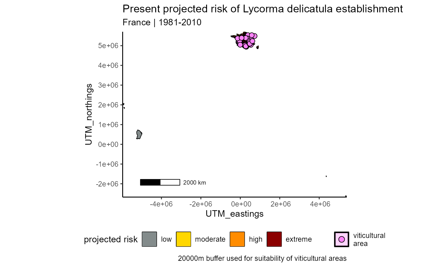
france_slf_risk_report[["risk_maps"]][["future_risk_map"]]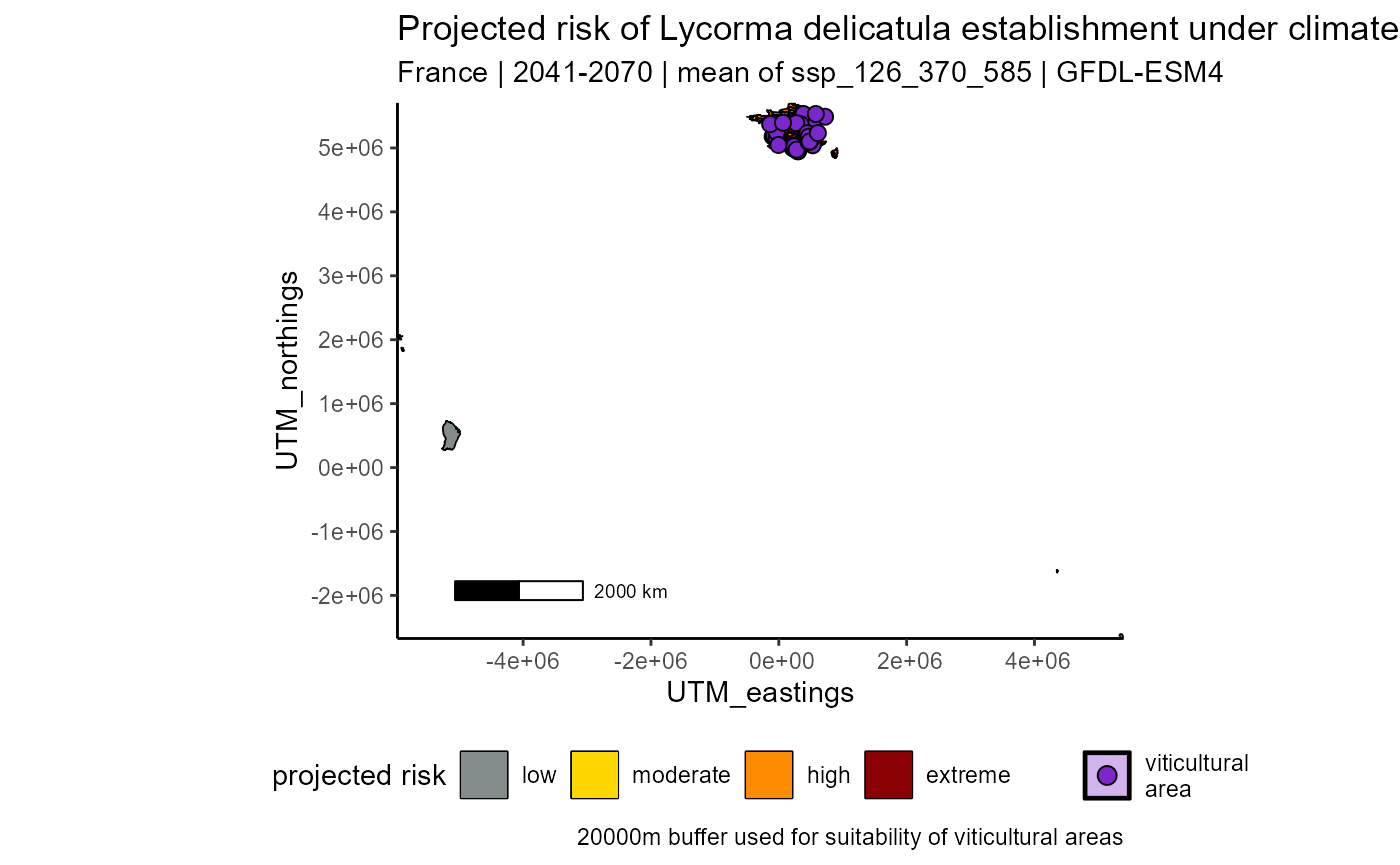
Unfortunately, the map did not format well because France possesses some territories outside its mainland. We can fix this with a few simple lines of code; we merely need to edit the axes of the plot:
france_current <- france_slf_risk_report[["risk_maps"]][["present_risk_map"]] +
  xlim(-482431.4012544825, 964862.802508965) +
  ylim(4804640.544946612, 5695846.383707797)
## Scale for x is already present.
## Adding another scale for x, which will replace the existing scale.
## Scale for y is already present.
## Adding another scale for y, which will replace the existing scale.
france_current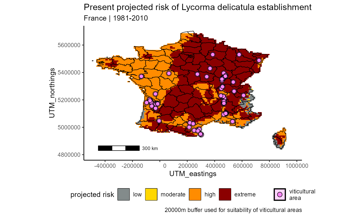
france_future <- france_slf_risk_report[["risk_maps"]][["future_risk_map"]] +
  xlim(-482431.4012544825, 964862.802508965) +
  ylim(4804640.544946612, 5695846.383707797)
## Scale for x is already present.
## Adding another scale for x, which will replace the existing scale.
## Scale for y is already present.
## Adding another scale for y, which will replace the existing scale.
france_future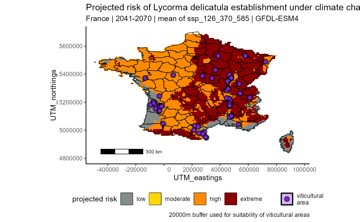
Now we can see the map of the mainland much better.
The next table shows the proportion of the map that is occupied by each risk level. This is a useful table to see how much of the viticultural area is at risk.
france_slf_risk_report[["risk_maps_prop_area_table"]]| model_suitability | area_km²_present | prop_area_present | area_km²_future | prop_area_future |
|---|---|---|---|---|
| unsuitable_agreement | 121,287 | 18% | 169,286 | 24.8% |
| regional | 214,079 | 31% | 250,768 | 36.8% |
| global | 801 | 0% | 1,069 | 0.2% |
| suitable_agreement | 346,052 | 51% | 261,097 | 38.3% |
| a future areas at risk calculated for period 2041-2070 | ||||
| a present risk calculated for period 1981-2010 |
Next, we have the viticultural risk plot, which shows the risk level of each winery in France. This is a useful plot to see the overall trend of how the wineries in France are changing risk over time. The arrows point from a vineyard in the present, to its risk in the future.
france_slf_risk_report[["viticultural_risk_plot"]]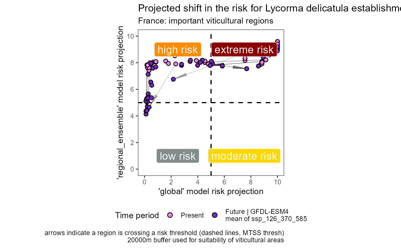
Next is the viticultural risk table, which shows a tally of the wineries at each risk level, both now and in the future. This is a useful table to see how many wineries are at each risk level, and how that changes over time. It serves to quantify the risk plot above. Negative numbers are decreasing in risk over time, and positive numbers are increasing in risk over time.
france_slf_risk_report[["viticultural_risk_table"]]| extreme_future | high_future | moderate_future | low_future | total_present | |
|---|---|---|---|---|---|
| extreme_present | 32 | -6 | 0 | 0 | 38 |
| high_present | +2 | 22 | 0 | -8 | 32 |
| moderate_present | +0 | +0 | 0 | 0 | 0 |
| low_present | +0 | +0 | +0 | 0 | 0 |
| total_future | 34 | 28 | 0 | 8 | 70 |
| a 20000m buffer used for suitability of viticultural areas | |||||
| a number signs indicate whether climate change is increasing or decreasing risk | |||||
| a present risk calculated for period 1981-2010 | |||||
| a future risk calculated for period 2041-2070 |
Next, we have a map of the shift in risk for SLF over time. Green areas will gain risk in the future, while blue areas will lose risk in the future. This is a useful map to see where SLF is expected to shift its range over time. The white areas remain consistently at risk over time, while the grey areas are never at risk.
france_slf_risk_report[["range_shift_map"]]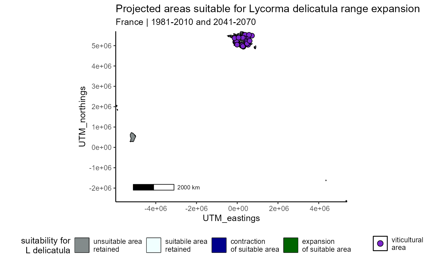
We cannot see this map well either; lets change the view on it.
france_shift <- france_slf_risk_report[["range_shift_map"]] +
  xlim(-482431.4012544825, 964862.802508965) +
  ylim(4804640.544946612, 5695846.383707797)
## Scale for x is already present.
## Adding another scale for x, which will replace the existing scale.
## Scale for y is already present.
## Adding another scale for y, which will replace the existing scale.
france_shift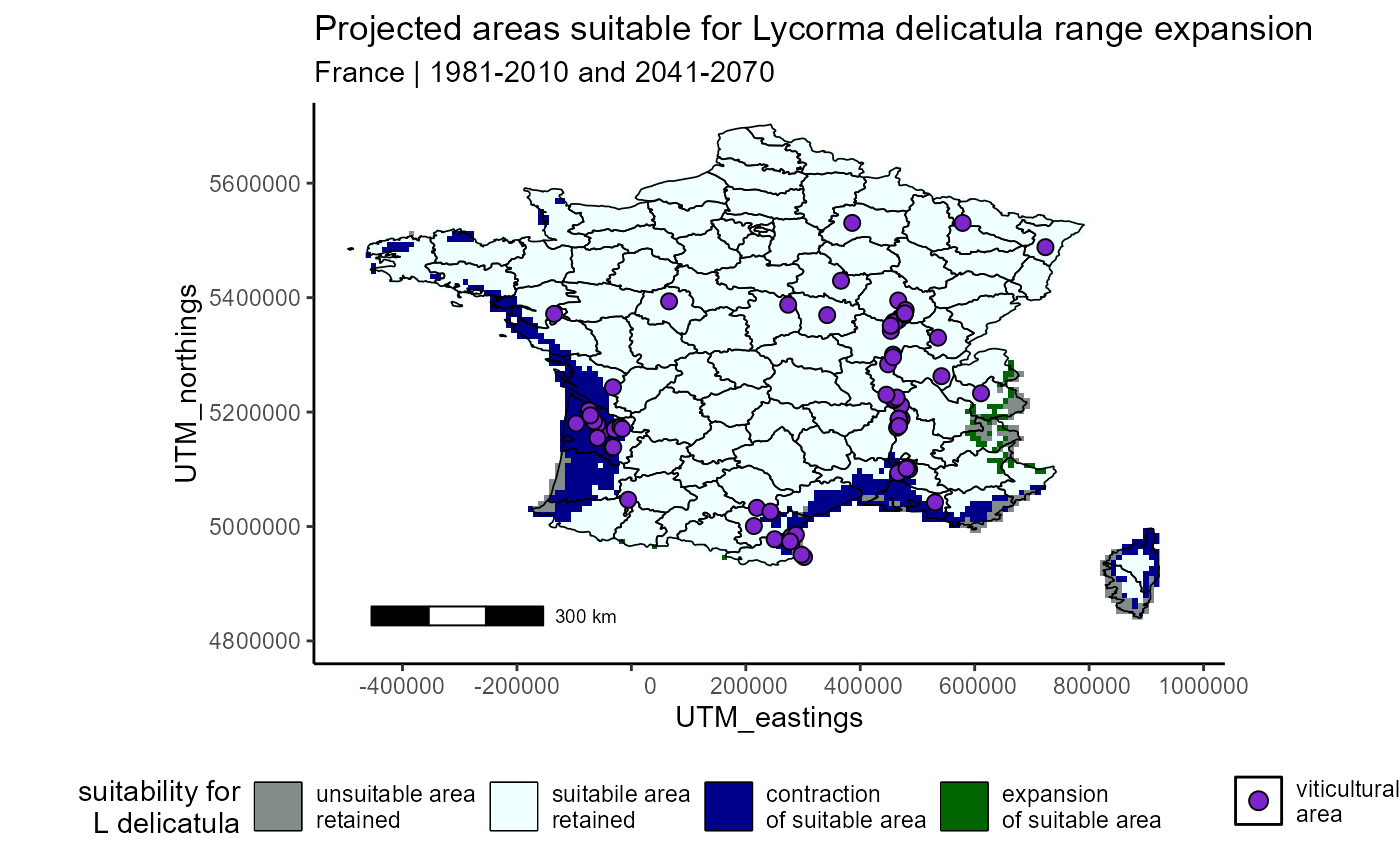
Finally, we havea table which calculates the total area for each of the categories in the above map.
france_slf_risk_report[["range_shift_table"]]| Ld_range_shift_type | area_km² | prop_total_area |
|---|---|---|
| remains_unsuitable | 116,835 | 17.1% |
| contraction | 52,451 | 7.7% |
| expansion | 4,453 | 0.7% |
| retained_suitability | 508,481 | 74.5% |
| a future areas at risk calculated for period 2041-2070 | ||
| a present risk calculated for period 1981-2010 |
Apply function to all possible countries
loop to apply function to wineries dataset
Primarily, I would like to use the wineries dataset to create a
report for each unique country on the list. Our winery records contain
64 unique countries that I will create reports for. These reports will
be saved to vignette-outputs/reports.
# import wineries dataset
IVR_locations <- readr::read_rds(file = file.path(here::here(), "data", "wineries_esri54017_tidied.rds"))


n_distinct(IVR_locations$Country)
## [1] 64
# there are 64 unique countries on the list

# get iso codes using rnaturalearth data
admin_0_countries <- read_sf(dsn = file.path(here::here(), "data-raw", "ne_countries", "ne_10m_admin_0_countries.shp")) %>%
  dplyr::select(ADMIN, ADM0_A3)

# replace names in sf
admin_0_countries$ADMIN <- stringr::str_replace_all(admin_0_countries$ADMIN, "United States of America", "United States")
admin_0_countries$ADMIN <- stringr::str_replace_all(admin_0_countries$ADMIN, "South Korea", "Republic of Korea")
admin_0_countries$ADMIN <- stringr::str_replace_all(admin_0_countries$ADMIN, "Palestine", "Palestinian territories")
admin_0_countries$ADMIN <- stringr::str_replace_all(admin_0_countries$ADMIN, "Cabo Verde", "Cape Verde")
admin_0_countries$ADMIN <- stringr::str_replace_all(admin_0_countries$ADMIN, "Czechia", "Czech Republic")
admin_0_countries$ADMIN <- stringr::str_replace_all(admin_0_countries$ADMIN, "Republic of Serbia", "Serbia")

# correct misspelling
IVR_locations$Country <- stringr::str_replace_all(IVR_locations$Country, "Algiera", "Algeria")

# join
IVR_locations_iso <- left_join(IVR_locations, admin_0_countries, join_by(Country == ADMIN)) %>%
  dplyr::rename("iso_a3" = "ADM0_A3")


# check
n_distinct(IVR_locations_iso$iso_a3)
## [1] 64
# it was successful, 64 unique iso codes

# sort dataset
unique_iso <- sort(unique(IVR_locations_iso$iso_a3))
# paired country names
unique_name <- IVR_locations_iso %>%
  group_by(iso_a3) %>%
  summarize(country = unique(Country)) %>%
  dplyr::select(country) %>%
  as.matrix() %>%
as.character()## [1] "Albania" "ALB"
## [1] "Argentina" "ARG"
## [1] "Armenia" "ARM"
## [1] "Australia" "AUS"
## [1] "Austria" "AUT"
## [1] "Azerbaijan" "AZE"
## [1] "Belgium" "BEL"
## [1] "Bulgaria" "BGR"
## [1] "Bosnia and Herzegovina" "BIH"
## [1] "Bolivia" "BOL"
## [1] "Brazil" "BRA"
## [1] "Canada" "CAN"
## [1] "Switzerland" "CHE"
## [1] "Chile" "CHL"
## [1] "China" "CHN"
## [1] "Cape Verde" "CPV"
## [1] "Cyprus" "CYP"
## [1] "Czech Republic" "CZE"
## [1] "Germany" "DEU"
## [1] "Algeria" "DZA"
## [1] "Spain" "ESP"
## [1] "France" "FRA"
## [1] "Georgia" "GEO"
## [1] "Greece" "GRC"
## [1] "Croatia" "HRV"
## [1] "Hungary" "HUN"
## [1] "Indonesia" "IDN"
## [1] "India" "IND"
## [1] "Ireland" "IRL"
## [1] "Iran" "IRN"
## [1] "Israel" "ISR"
## [1] "Italy" "ITA"
## [1] "Japan" "JPN"
## [1] "Republic of Korea" "KOR"
## [1] "Lebanon" "LBN"
## [1] "Lithuania" "LTU"
## [1] "Luxembourg" "LUX"
## [1] "Latvia" "LVA"
## [1] "Morocco" "MAR"
## [1] "Moldova" "MDA"
## [1] "Mexico" "MEX"
## [1] "North Macedonia" "MKD"
## [1] "Myanmar" "MMR"
## [1] "Montenegro" "MNE"
## [1] "Netherlands" "NLD"
## [1] "New Zealand" "NZL"
## [1] "Peru" "PER"
## [1] "Poland" "POL"
## [1] "Portugal" "PRT"
## [1] "Palestinian territories" "PSX"
## [1] "Romania" "ROU"
## [1] "Russia" "RUS"
## [1] "Serbia" "SRB"
## [1] "Slovakia" "SVK"
## [1] "Slovenia" "SVN"
## [1] "Sweden" "SWE"
## [1] "Syria" "SYR"
## [1] "Tunisia" "TUN"
## [1] "Turkey" "TUR"
## [1] "Ukraine" "UKR"
## [1] "United States" "USA"
## [1] "Venezuela" "VEN"
## [1] "Vietnam" "VNM"
## [1] "South Africa" "ZAF"
length(unique_name)## [1] 64We ran checks and everything seems correct. Above is a list of
countries that will get a report, 64 in total. Now, I will run a loop to
create those reports and save the, to
root/vignette-outputs/reports.
# loop thru country iso codes and names together
for (a in seq_along(unique_iso)) {

  scari::create_risk_report(
    locality.iso = unique_iso[a], # iso codes
    locality.name = unique_name[a], # names
    locality.type = "country",
    mypath = file.path(here::here(), "vignette-outputs", "reports", unique_name[a]),
    create.dir = TRUE, # create subdirectory for plots
    save.report = TRUE,
    buffer.dist = 20000 # distance at which buffers should be drawn on maps to indicate IVR suitability predictions
    )

}
Some of these maps might need to be edited to zoom in on the countries, because some countries have geographically separated territories that are not relevant to the analysis. The code to zoom in on those plots will be in the following section.