How to use this project
1. Produce localized reports on SLF risk to viticulture
Our primary datasets, including risk maps and a viticultural risk
analysis, can be accessed by executing the function
create_risk_report(). This function creates a localized (at
the country or state/provincial level) report of the risk for
Lycorma delicatula to local viticulture. It can be applied to
globally important wine growing regions because it uses our dataset
data/wineries_esri54017_tidied.rds, which contains a sample
(1,072) of the world’s most important wine growing regions. Users can
and should apply this function for their locality as we are projecting
that the risk of Lycorma delicatula establishment will expand
under climate change. Lycorma delicatula has been classified as
being capable of (global) pan-invasion and viticulure has already been
devastated in some regions, so there is high potential for viticultural
damage under climate change (Huron et al, 2022).
In this vignette, I will give an example of how this function can be
applied to both a country and state/province to assess risk at different
scales. For a more complete example of the usage of the
create_risk_report() function and all of its outputs, see
the vignette 150_create_risk_report_example_usage.
Our function recreates major data sets that we provide in our main analysis, including:
- list of known important wine regions within the locality with predicted suitability values and levels
- current and future risk maps for SLF establishment
- range shift map of potential range expansion for L. delicatula under climate change
- Viticultural quadrant plot depicting of the risk for SLF establishment for known wine regions within the locality. This plot depicts the intersection of our two modeled scales.
- risk table quantifying the level of risk to vineyards according to the quadrant plot
Here is an example of a workflow for creating a localized risk map and how this might be applied. I will give an example of how I might interpret the risk for Lycorma delicatula establishment in the United States, and then I will show how to narrow its scope to a more localized region, Washington State.
I might begin by creating a report at the national level. To create this, you will need the alpha-3 iso country code.
scari::create_risk_report(
  locality.iso = "usa",
  locality.type = "country", # to specify the type of report
  buffer.dist = 20000, # in meters, this is the buffer zone defining the viticultural area
  create.dir = FALSE, # should a directory be created for the report? If TRUE, param mypath will be required
  save.report = FALSE # should the report be saved?
)
You should first note the three most important outputs of this function:
- the risk maps
- the accompanying viticultural risk quadrant plot
- tabled list of viticultural regions in this locality
First, we observe the risk map, which depicts the risk of SLF establishment using the agreement between our regional-scale model ensemble and our global-scale model. More agreement on suitability mean higher risk.
USA_current <- usa_slf_risk_report[["risk_maps"]][["present_risk_map"]] +
  # you may need to crop the map due to outlying territories, as we have done here
  xlim(-12060785.03, -6271608.22) + # the boundaries in UTM
  ylim(3091555.56, 5614050.10)

USA_current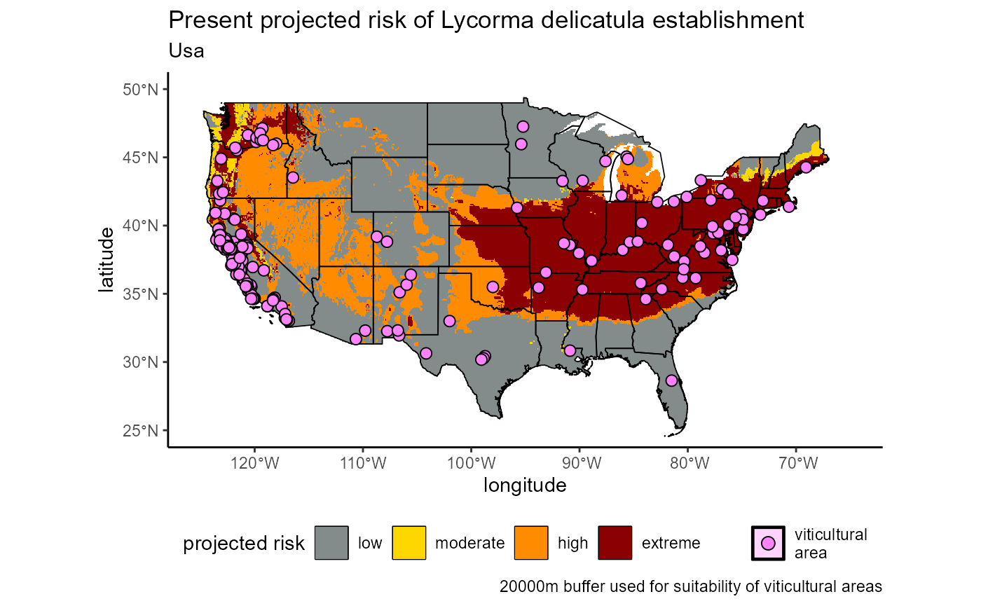
Fig 1. Projected current risk of Lycorma delicatula establishment | USA
USA_future <- usa_slf_risk_report[["risk_maps"]][["future_risk_map"]] +
  # you may need to crop the map due to outlying territories, as we have done here
  xlim(-12060785.03, -6271608.22) + # the boundaries in UTM
  ylim(3091555.56, 5614050.10)

USA_future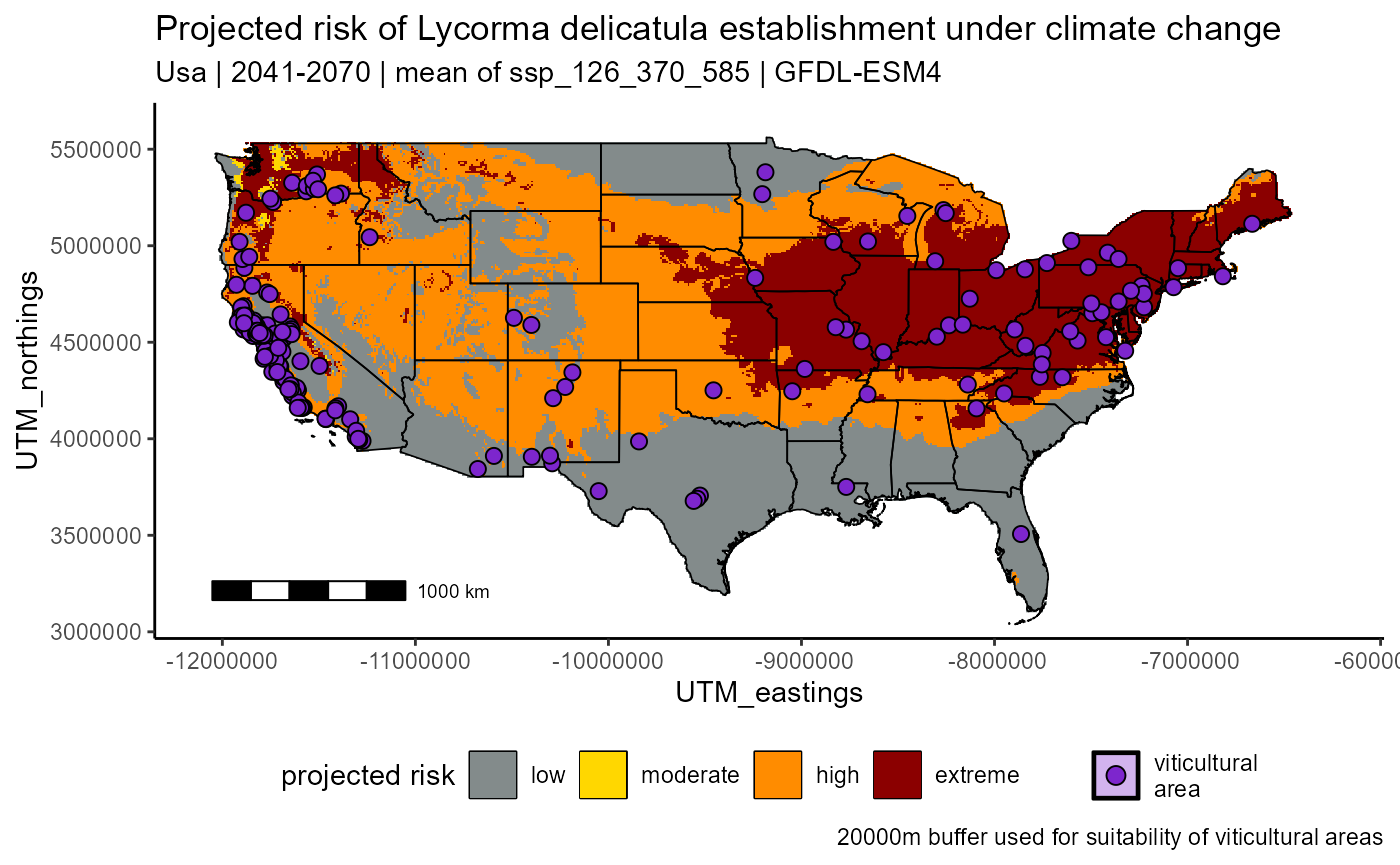
Fig 2. Projected future risk of Lycorma delicatula establishment under climate change | USA
The points on the map represent key viticultural regions. We have extracted the suitability of each viticultural region and depicted its quantitative shift in risk on our second output, the viticultural risk quadrant plot. This plot quantifies the level of risk along both modeled scales, both presently (light purple) and in the future (dark purple) under a predicted climate change shift (arrows):
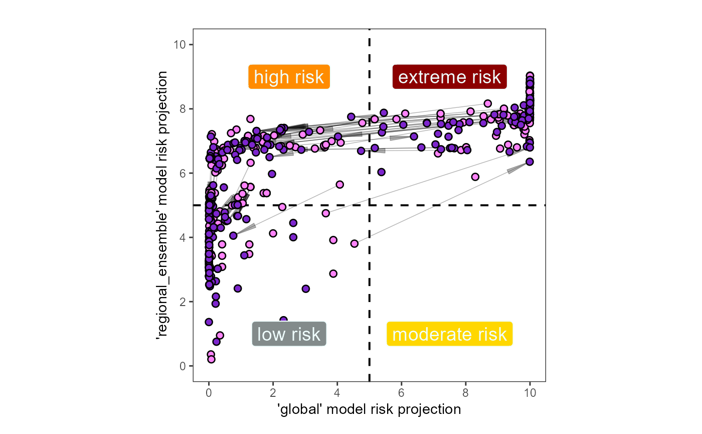
Fig. 3: Projected shift in the risk for Lycorma delicatula establishment at key viticultural regions due to climate change | USA
The accompanying table provides a list of key viticultural regions and their geographical region (state/province), with predicted risk levels:
Table 1: List of viticultural regions and their projected risk
You may begin to notice that a particular region has many records, like we can see is the case for Washington State. You could then produce a report only for that region, to get a better idea of the overall trend of risk shift due to climate change. We will produce a report for Washington State alone, to better visualize this trend:
scari::create_risk_report(
  locality.iso = "usa", # the country iso is still required
  locality.name = "washington", # the name must be specified
  locality.type = "state_province", # we have changed the report type
  buffer.dist = 20000, # in meters
  create.dir = FALSE,
  save.report = FALSE
)
We can see that most of Washington is at some level of SLF risk presently. Under climate change, risk is projected to decrease some, but one or both modeled scales still predict that SLF can establish in most of the state.
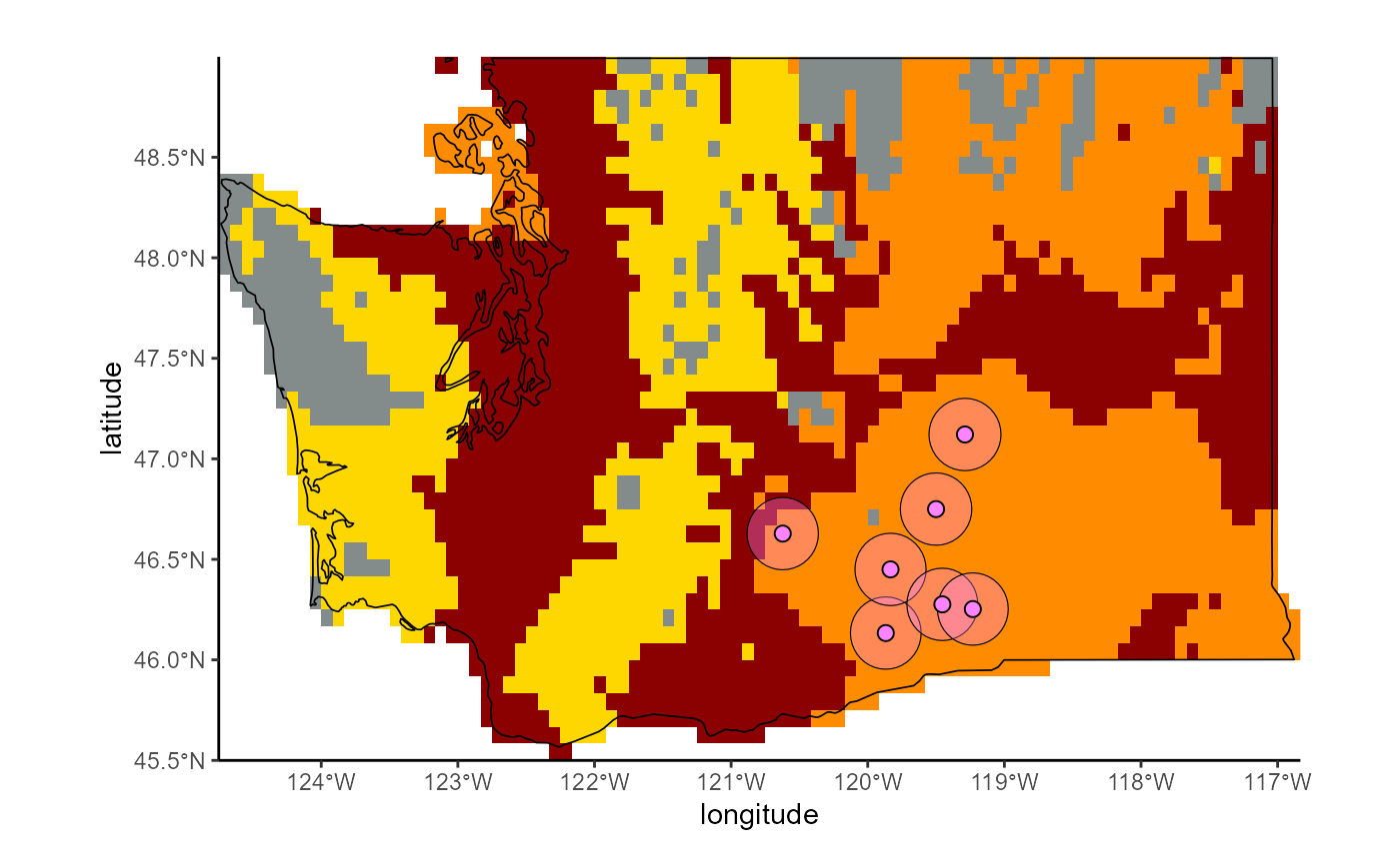
Fig. 3: Projected current risk of Lycorma delicatula establishment | Washington, USA
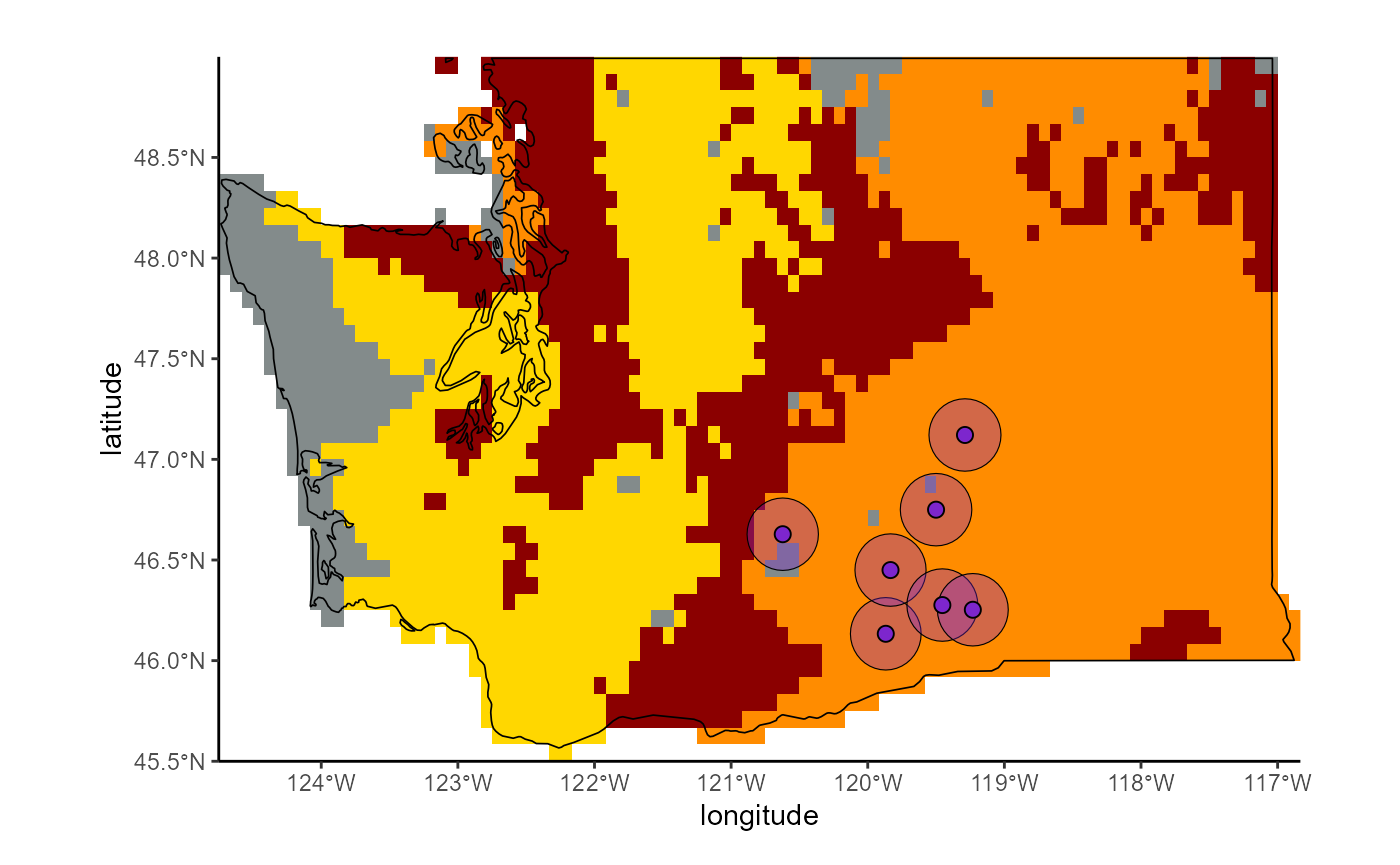
Fig. 4: Projected future risk of Lycorma delicatula establishment under climate change | Washington, USA
Based on the viticultural risk quadrant plot, we can now see that Washington state exhibits a totally different trend from the rest of the country. While viticultural regions across the united states exhibit a range of risk levels, regions in Washington are either at high or extreme risk for SLF establishment, and this pattern does not change under predicted climate change levels.
Note At this scale, we can see the buffer zones used to assess viticultural region risk.
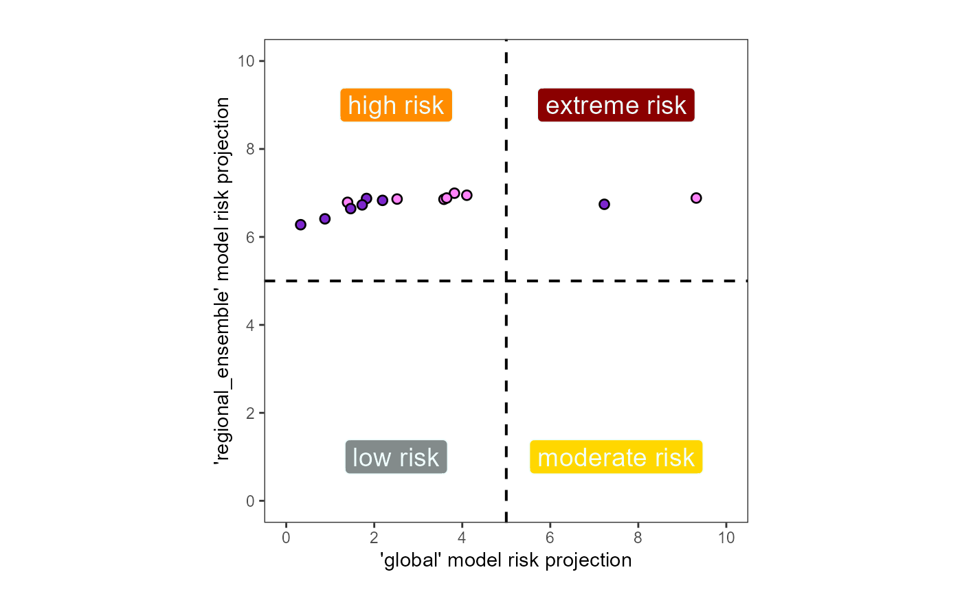
Fig. 5: Projected shift in the risk for Lycorma delicatula establishment at key viticultural regions due to climate change | Washington, USA
In our more localized analysis, we might also be interested in
quantifying the total area at risk for SLF or the total number of
viticultural regions at risk for SLF establishment. For this, we will
look at two additional outputs from
create_risk_report():
- risk map area table- this quantifies the areas and proportions of the total occupied by each risk category on the risk map
- viticultural risk table- this quantifies the number of winegrowing regions that are projected to fall into each risk category, both now and in the future under climate change
First, let’s look at the risk map area table:
Table 2: Table quantifying the projected current and future suitable area for Lycorma delicatula establishment | Washington, USA
| model_suitability | area_km²_present | prop_area_present | area_km²_future | prop_area_future |
|---|---|---|---|---|
| unsuitable_agreement | 25,558 | 13.4% | 18,968 | 10.0% |
| regional | 61,445 | 32.3% | 61,267 | 32.2% |
| global | 9,261 | 4.9% | 15,673 | 8.2% |
| suitable_agreement | 93,860 | 49.4% | 94,216 | 49.6% |
| a future areas at risk calculated for period 2041-2070 | ||||
| a present risk calculated for period 1981-2010 |
We can see from this table that the total unsuitable area decreased under climate change, from 8.6% to 7.4%, but this change was mostly found in the regional-scale model ensemble, which predicted ~9% more suitable arae under climate change. Our modeled scales also diverged in the agreed suitable area (suitable_agreement decreased by ~9%).
Next, lets look at the viticultural risk table:
Table 3: Table quantifying the projected shift in the risk for Lycorma delicatula establishment at key viticultural regions due to climate change | Washington, USA
| extreme_future | high_future | moderate_future | low_future | total_present | |
|---|---|---|---|---|---|
| extreme_present | 0 | 0 | 0 | 0 | 0 |
| high_present | +0 | 7 | 0 | 0 | 7 |
| moderate_present | +0 | +0 | 0 | 0 | 0 |
| low_present | +0 | +0 | +0 | 0 | 0 |
| total_future | 0 | 7 | 0 | 0 | 7 |
| a 20000m buffer used for suitability of viticultural areas | |||||
| a number signs indicate whether climate change is increasing or decreasing risk | |||||
| a present risk calculated for period 1981-2010 | |||||
| a future risk calculated for period 2041-2070 |
From this table, we can see that all 7 viticultural regions maintain their present risk level under climate change. Six regions fall into the high risk category (regional ensemble suitability only) and one falls into the extreme risk category (suitable area agreement).
Users should explore the other localities and data types available with this function.
2. Recreate the analysis for another invasive species of interest
For modelers who wish to apply this pipeline for other invasive species, this pipeline can easily be adapted to model the risk of establishment by simply changing the input datasets and modeled scales.
First, a modeler would need to change the input datasets, outlined in
vignettes 020-040. In vignette 020, I retrieved input data from GBIF,
which hosts datasets for thousands of other species. I recommend
including extra data from other databases and the literature as I did in
my analysis, but GBIF is a great starting point for data retrieval. Here
is an example using the package rgbif. Before I perform
this operation, I will need to enter my user credentials for gbif; to
keep these private, I will edit the .Renviron and call them from there.
Once this chunk is run and the .Renviron pops up, enter your username,
password and email credentials in the following format on lines 1-3:
- GBIF_USER=” ”
- GBIF_PWD=” ”
- GBIF_EMAIL=” ”
# edit R environment for user credentials
usethis::edit_r_environ()
Save and close the document, and restart R. Now I will search for species occurrence records using GBIF.
slf_id <- rgbif::occ_search(scientificName = "Lycorma delicatula")[["data"]]

slf_id <- slf_id %>%
  dplyr::select(taxonKey) %>%
  dplyr::slice_head() %>%
  as.character()


# initiate download
records_gbif <- rgbif::occ_download(
  # general formatting
  type = "and",
  format = "SIMPLE_CSV",
  # inclusion rules
  pred("taxonKey", slf_id), # search by GBIF ID, not species name
  pred("hasCoordinate", TRUE),
  pred("hasGeospatialIssue", FALSE),
  pred("occurrenceStatus", "PRESENT")
)
The input covariates would also need to change based on what is biologically relevant for the particular species. I outline the process of choosing input covariates in vignette 030.
Once the input data have been adapted to the user’s needs, the
regional-scale models will need to be applied per region of interest.
Each regional-scale model depends on a spcecific background area
selection for MaxEnt that will need to change. I outline the process for
choosing this area in vignette 060, in which I subset the presence data
by region and intersect these subsets with the Köppen-Geiger climate
zones to select the appropriate background area. This resulting polygon
would need to be cropped to the region of interest. I use the
kgc, terra, and sf packages for
this analysis:
# get K-G zones
kmz_data <- kgc::kmz

# generate coordinates
kmz_lat <- kgc::genCoords(latlon = "lat", full = TRUE)
kmz_lon <- kgc::genCoords(latlon = "lon", full = TRUE)

# join data and coordinates
kmz_data <- cbind(kmz_lat, kmz_lon) %>%
  cbind(., kmz_data) %>%
  as.data.frame() %>%
  # relocate column
  dplyr::select(kmz_lon, everything())

# convert to raster
KG_zones_rast <- terra::rast(
  x = kmz_data,
  type = "xyz",
  crs = "EPSG:4326"
  )

# reproject to ESRI:54017
kmz_data_rast <- terra::project(
  x = kmz_data_rast,
  y = "ESRI:54017",
  method = "bilinear", # bilinear interpolation for continuous data
  threads = TRUE # use multiple threads for faster processing
)

# next, convert raster to polygon
KG_zones_poly <- terra::as.polygons(
  x = KG_zones_rast,
  aggregate = TRUE, # combine cells with the same value into one area
  values = TRUE, # include cell values as attributes
  crs = "ESRI:54017"
)
KG_zones_poly <- sf::st_as_sf(KG_zones_poly)

# intersect polygon and presences
regional_poly <- sf::st_filter(x = KG_zones_poly, y = presence_data)
Once the presence data, covariate data and background points have been chosen, the user might apply this framework for any invasive species and ensemble models for any region of interest.
References
Bryant, C., Wheeler, N. R., Rubel, F., & French, R. H. (2017). kgc: Koeppen-Geiger Climatic Zones. https://CRAN.R-project.org/package=kgc
Chamberlain S, Barve V, Mcglinn D, Oldoni D, Desmet P, Geffert L, Ram K (2024). rgbif: Interface to the Global Biodiversity Information Facility API. R package version 3.8.0, https://CRAN.R-project.org/package=rgbif.
Gallien, L., Douzet, R., Pratte, S., Zimmermann, N. E., & Thuiller, W. (2012). Invasive species distribution models – how violating the equilibrium assumption can create new insights. Global Ecology and Biogeography, 21(11), 1126–1136. https://doi.org/10.1111/j.1466-8238.2012.00768.x
Huron, N. A., Behm, J. E., & Helmus, M. R. (2022). Paninvasion severity assessment of a U.S. grape pest to disrupt the global wine market. Communications Biology, 5(1), 655. https://doi.org/10.1038/s42003-022-03580-w
Pebesma, E., 2018. Simple Features for R: Standardized Support for Spatial Vector Data. The R Journal 10 (1), 439-446, https://doi.org/10.32614/RJ-2018-009
Phillips, S. J., Anderson, R. P., & Schapire, R. E. (2006). Maximum entropy modeling of species geographic distributions. Ecological Modelling, 190(3), 231–259. https://doi.org/10.1016/j.ecolmodel.2005.03.026
Hijmans R (2024). terra: Spatial Data Analysis. R package version 1.7-81, https://rspatial.github.io/terra/, https://rspatial.org/.
Ushey K, Wickham H (2024). renv: Project Environments. R package version 1.0.7, https://github.com/rstudio/renv, https://rstudio.github.io/renv/.
Wickham H, Averick M, Bryan J, Chang W, McGowan LD, François R, Grolemund G, Hayes A, Henry L, Hester J, Kuhn M, Pedersen TL, Miller E, Bache SM, Müller K, Ooms J, Robinson D, Seidel DP, Spinu V, Takahashi K, Vaughan D, Wilke C, Woo K, Yutani H (2019). “Welcome to the tidyverse.” Journal of Open Source Software, 4(43), 1686. doi:10.21105/joss.01686.