Ensemble regional-scale models using a weighted mean

Overview

In vignettes 060-090, I created three regional-scale MaxEnt models for invasive plant pest Lycorma delicatula based on historical and predicted future climate trends under climate change. One of these models was based on the planthopper’s native range in east Asia, while the other two models were based on the regions it has so far invaded (the Koreas/Japan and North America). These regional models were created using the same data and settings as the global-scale version (vignette 050), which considers all regions together.

Our goal is to compare the global-scale output with that from the three regional-scale models. A global-scale model is the traditional approach to modeling species distributions and represents an important generalization made using all data, but it may not consider localized climate conditions that differ between regions (Gallien et al, 2012). I hypothesized that by creating models at multiple spatial scales, I can have more confidence in suitability predictions made for specific SLF populations and important viticultural regions, and can predict the risk of specific populations spreading now and under climate change (Araújo and New, 2007). I also hypothesize that the regional-scale models, once ensembled into a single prediction, will make more refined predictions than a global-scale model could.

We will ensemble the three regional-scale models into a single prediction using a weighted mean approach. This will involve weighting each model’s predictions by the ExDet metric (Which we measured in the last vignette, 100) and its test AUC value. The ExDet metric measures the level of extrapolation in the model’s predictions when projecting models. Measuring the level of extrapolation is very important when making predictions across different climate zones, time periods, or for range shifting species (we check all of those boxes) (Elith et al, 2010; Mesgaran et al, 2014). We will directly use the Exdet metric from each model to measure our confidence in its predictions for a particular grid cell. We will also use the test AUC from each model in the weighting so that we also consider goodness of fit.

Setup

library(tidyverse)

library(here) 
# here() is set at the root folder of this package

# spatial data handling
library(terra)

# aesthetics
library(ggnewscale)

Note: I will be setting the global options of this document so that only certain code chunks are rendered in the final .html file. I will set the eval = FALSE so that none of the code is re-run (preventing files from being overwritten during knitting) and will simply overwrite this in chunks with plots.

dir.create(path = file.path(mypath, "models", "slf_regional_ensemble_v1"))
dir.create(path = file.path(mypath, "models", "slf_regional_ensemble_v1", "plots"))

Plotting

I will define a helper function and import the background area rasters for plotting.

format_decimal <- function(x) as.numeric(sprintf("%.*f", 2, x))
# formats decimals to 2 places

# path to directory
mypath <- file.path(here::here() %>% 
                       dirname(),
                     "maxent/historical_climate_rasters/chelsa2.1_30arcsec")


# native
regional_native_background_area <- terra::rast(x = file.path(mypath, "v1_maxent_10km", "bio11_1981-2010_regional_native_KG.asc"))
# invaded
regional_invaded_background_area <- terra::rast(x = file.path(mypath, "v1_maxent_10km", "bio11_1981-2010_regional_invaded_KG.asc"))
# invaded_asian
regional_invaded_asian_background_area <- terra::rast(x = file.path(mypath, "v1_maxent_10km", "bio11_1981-2010_regional_invaded_asian_KG.asc"))


# convert to df
regional_native_background_area_df <- terra::as.data.frame(regional_native_background_area, xy = TRUE)
regional_invaded_background_area_df <- terra::as.data.frame(regional_invaded_background_area, xy = TRUE)
regional_invaded_asian_background_area_df <- terra::as.data.frame(regional_invaded_asian_background_area, xy = TRUE)

1. Import datasets

1.1 MaxEnt Predictions

First, I need to load in the rasters containing the predictions from each model. I will load in both the historical and climate change versions of these predictions.

# output directory
mypath <- file.path(here::here() %>% 
                       dirname(),
                     "maxent")

pred_regional_native <- terra::rast(
  x = file.path(mypath, "models", "slf_regional_native_v3", "regional_native_pred_suit_clamped_cloglog_globe_1981-2010.asc")
)

# CMIP6
# SSP126
pred_regional_native_126 <- terra::rast(
  x = file.path(mypath, "models", "slf_regional_native_v3", "regional_native_pred_suit_clamped_cloglog_globe_2041-2070_GFDL_ssp126.asc")
)

# SSP370
pred_regional_native_370 <- terra::rast(
  x = file.path(mypath, "models", "slf_regional_native_v3", "regional_native_pred_suit_clamped_cloglog_globe_2041-2070_GFDL_ssp370.asc")
)

# SSP585
pred_regional_native_585 <- terra::rast(
  x = file.path(mypath, "models", "slf_regional_native_v3", "regional_native_pred_suit_clamped_cloglog_globe_2041-2070_GFDL_ssp585.asc")
)

pred_regional_invaded <- terra::rast(
  x = file.path(mypath, "models", "slf_regional_invaded_v7", "regional_invaded_pred_suit_clamped_cloglog_globe_1981-2010.asc")
)

# CMIP6
# SSP126
pred_regional_invaded_126 <- terra::rast(
  x = file.path(mypath, "models", "slf_regional_invaded_v7", "regional_invaded_pred_suit_clamped_cloglog_globe_2041-2070_GFDL_ssp126.asc")
)

# SSP370
pred_regional_invaded_370 <- terra::rast(
  x = file.path(mypath, "models", "slf_regional_invaded_v7", "regional_invaded_pred_suit_clamped_cloglog_globe_2041-2070_GFDL_ssp370.asc")
)

# SSP585
pred_regional_invaded_585 <- terra::rast(
  x = file.path(mypath, "models", "slf_regional_invaded_v7", "regional_invaded_pred_suit_clamped_cloglog_globe_2041-2070_GFDL_ssp585.asc")
)

pred_regional_invaded_asian <- terra::rast(
  x = file.path(mypath, "models", "slf_regional_invaded_asian_v2", "regional_invaded_asian_pred_suit_clamped_cloglog_globe_1981-2010.asc")
)

# CMIP6
# SSP126
pred_regional_invaded_asian_126 <- terra::rast(
  x = file.path(mypath, "models", "slf_regional_invaded_asian_v2", "regional_invaded_asian_pred_suit_clamped_cloglog_globe_2041-2070_GFDL_ssp126.asc")
)

# SSP370
pred_regional_invaded_asian_370 <- terra::rast(
  x = file.path(mypath, "models", "slf_regional_invaded_asian_v2", "regional_invaded_asian_pred_suit_clamped_cloglog_globe_2041-2070_GFDL_ssp370.asc")
)


# SSP585
pred_regional_invaded_asian_585 <- terra::rast(
  x = file.path(mypath, "models", "slf_regional_invaded_asian_v2", "regional_invaded_asian_pred_suit_clamped_cloglog_globe_2041-2070_GFDL_ssp585.asc")
)

1.2 AUC values

Next, I will load in the AUC value from each model, which will be used to weight each model’s predictions, specifically based on its test AUC value.

AUC_regional_native <- read_csv(file = file.path(mypath, "models", "slf_regional_native_v3", "regional_native_AUC_TSS.csv")) %>%
  dplyr::select(AUC) %>%
  dplyr::slice(2) %>%
  as.numeric()

AUC_regional_invaded <- read_csv(file = file.path(mypath, "models", "slf_regional_invaded_v7", "regional_invaded_AUC_TSS.csv")) %>%
  dplyr::select(AUC) %>%
  dplyr::slice(2) %>%
  as.numeric()

AUC_regional_invaded_asian <- read_csv(file = file.path(mypath, "models", "slf_regional_invaded_asian_v2", "regional_invaded_asian_AUC_TSS.csv")) %>%
  dplyr::select(AUC) %>%
  dplyr::slice(2) %>%
  as.numeric()

AUC_values <- tibble(
  model = c("AUC_regional_native", "AUC_regional_invaded", "AUC_regional_invaded_asian"),
  AUC_value = c(AUC_regional_native, AUC_regional_invaded, AUC_regional_invaded_asian)
)

1.3 ExDet rasters

Finally, I will load in the results from the ExDet analysis to weight the ensemble.

exdet_regional_native <- terra::rast(
  x = file.path(mypath, "models", "slf_regional_native_v3", "ExDet_slf_regional_native_v3_background_projGlobe.tif")
)

# CMIP6
# SSP126
exdet_regional_native_126 <- terra::rast(
  x = file.path(mypath, "models", "slf_regional_native_v3", "ExDet_slf_regional_native_v3_background_projGlobe_2041-2070_ssp126_GFDL.tif")
)

# SSP370
exdet_regional_native_370 <- terra::rast(
  x = file.path(mypath, "models", "slf_regional_native_v3", "ExDet_slf_regional_native_v3_background_projGlobe_2041-2070_ssp370_GFDL.tif")
)

# SSP585
exdet_regional_native_585 <- terra::rast(
  x = file.path(mypath, "models", "slf_regional_native_v3", "ExDet_slf_regional_native_v3_background_projGlobe_2041-2070_ssp585_GFDL.tif")
)

exdet_regional_invaded <- terra::rast(
  x = file.path(mypath, "models", "slf_regional_invaded_v7", "ExDet_slf_regional_invaded_v7_background_projGlobe.tif")
)

# CMIP6
# SSP126
exdet_regional_invaded_126 <- terra::rast(
  x = file.path(mypath, "models", "slf_regional_invaded_v7", "ExDet_slf_regional_invaded_v7_background_projGlobe_2041-2070_ssp126_GFDL.tif")
)

# SSP370
exdet_regional_invaded_370 <- terra::rast(
  x = file.path(mypath, "models", "slf_regional_invaded_v7", "ExDet_slf_regional_invaded_v7_background_projGlobe_2041-2070_ssp370_GFDL.tif")
)

# SSP585
exdet_regional_invaded_585 <- terra::rast(
  x = file.path(mypath, "models", "slf_regional_invaded_v7", "ExDet_slf_regional_invaded_v7_background_projGlobe_2041-2070_ssp585_GFDL.tif")
)

exdet_regional_invaded_asian <- terra::rast(
  x = file.path(mypath, "models", "slf_regional_invaded_asian_v2", "ExDet_slf_regional_invaded_asian_v2_background_projGlobe.tif")
)


# CMIP6
# SSP126
exdet_regional_invaded_asian_126 <- terra::rast(
  x = file.path(mypath, "models", "slf_regional_invaded_asian_v2", "ExDet_slf_regional_invaded_asian_v2_background_projGlobe_2041-2070_ssp126_GFDL.tif")
)

# SSP370
exdet_regional_invaded_asian_370 <- terra::rast(
  x = file.path(mypath, "models", "slf_regional_invaded_asian_v2", "ExDet_slf_regional_invaded_asian_v2_background_projGlobe_2041-2070_ssp370_GFDL.tif")
)

# SSP585
exdet_regional_invaded_asian_585 <- terra::rast(
  x = file.path(mypath, "models", "slf_regional_invaded_asian_v2", "ExDet_slf_regional_invaded_asian_v2_background_projGlobe_2041-2070_ssp585_GFDL.tif")
)

2. Edit import datasets

2.1 Stack rasters

I will need to stack the predicted and ExDet rasters to perform this analysis.

pred_hist_stack <- c(pred_regional_native, pred_regional_invaded, pred_regional_invaded_asian)

# CMIP6
pred_126_stack <- c(pred_regional_native_126, pred_regional_invaded_126, pred_regional_invaded_asian_126)
pred_370_stack <- c(pred_regional_native_370, pred_regional_invaded_370, pred_regional_invaded_asian_370)
pred_585_stack <- c(pred_regional_native_585, pred_regional_invaded_585, pred_regional_invaded_asian_585)

exdet_hist_stack <- c(exdet_regional_native, exdet_regional_invaded, exdet_regional_invaded_asian)

# CMIP6
exdet_126_stack <- c(exdet_regional_native_126, exdet_regional_invaded_126, exdet_regional_invaded_asian_126)
exdet_370_stack <- c(exdet_regional_native_370, exdet_regional_invaded_370, exdet_regional_invaded_asian_370)
exdet_585_stack <- c(exdet_regional_native_585, exdet_regional_invaded_585, exdet_regional_invaded_asian_585)

2.2 Preparatory raster edits

The pred rasters need to be cropped slightly because the function used to create the ExDet rasters cropped them slightly. These raster sets need to share the same extent for downstream manipulations.

terra::ext(pred_hist_stack)
terra::ext(exdet_hist_stack)


# I will trim the rasters to the extent of the exdet rasters
ext.obj <- terra::ext(-180.00013888885, 178.999859675084, -58.5001390148238, 82.99986041915)

# crop rasters
pred_hist_stack <- terra::crop(pred_hist_stack, ext.obj)
# CMIP6
pred_126_stack <- terra::crop(pred_126_stack, ext.obj)
pred_370_stack <- terra::crop(pred_370_stack, ext.obj)
pred_585_stack <- terra::crop(pred_585_stack, ext.obj)

names(pred_hist_stack) <- c("pred_regional_native", "pred_regional_invaded", "pred_regional_invaded_asian")
# CMIP6
names(pred_126_stack) <- c("pred_regional_native_126", "pred_regional_invaded_126", "pred_regional_invaded_asian_126")
names(pred_370_stack) <- c("pred_regional_native_370", "pred_regional_invaded_370", "pred_regional_invaded_asian_370")
names(pred_585_stack) <- c("pred_regional_native_585", "pred_regional_invaded_585", "pred_regional_invaded_asian_585")

Now, I need to prepare to weight the predicted distribution rasters using their respective ExDet raster.

3. Ensemble rasters

I will create a weight factor for each model raster in this section across several steps. First, I will convert the ExDet rasters to a weight value. Next, I will add the test AUC values to these rasters and create a weighting factor. Finally, I will apply the weights to take the weighted mean of the three models.

3.1 Format ExDet rasters into weighting factor

First, I will need to manipulate the ExDet rasters so they can be used for weighting. I will begin by adding 1 to any negative ExDet value and then taking the absolute value of each cell. This way, the weighting is performed on a positive scale. The ExDet metric works such that anything between 0 and 1 is not extrapolated, while anything below 0 or above 1 is extrapolated. Next, I will convert any ExDet value below 0 to 1, so that cells without extrapolation are simply not weighted.

Add 1 to any negative ExDet values
Take abs value of ExDet values
Convert any ExDet value below 1 to 1
Take reciprocal of ExDet raster values

historical

# 1. add 1 to negatives

# take minmax before
minmax(exdet_hist_stack)

# the min values of each layer should be -1.4, -2.79 and -2.5 respectively after ifelse
# the max values should be unchanged at 1.4, 1.22 and 2.2

exdet_hist_stack <- terra::ifel(
  exdet_hist_stack < 0, # if the value is < 0
  exdet_hist_stack - 1, # subtract 1
  exdet_hist_stack # else, keep the same
  )

# minmax after
minmax(exdet_hist_stack)


# 2. take abs

exdet_hist_stack <- abs(exdet_hist_stack)

minmax(exdet_hist_stack)


# 3. convert values below 1 to 1

exdet_hist_stack <- terra::ifel(
  exdet_hist_stack < 1, # if the value is < 1 or == 0
  1, # make 1
  exdet_hist_stack # else, keep the same
  )

minmax(exdet_hist_stack)


# 4. take reciprocals

exdet_hist_stack <- terra::app(exdet_hist_stack, fun = (function(i) 1 / i))

minmax(exdet_hist_stack)

terra::writeRaster(
  x = exdet_hist_stack, 
  filename = c(
    file.path(mypath, "models", "working_dir", "exdet_weights_slf_regional_native_v3.tif"),
    file.path(mypath, "models", "working_dir", "exdet_weights_slf_regional_invaded_v7.tif"),
    file.path(mypath, "models", "working_dir", "exdet_weights_slf_regional_invaded_asian_v2.tif")
  ),
  filetype = "GTiff",
  overwrite = FALSE
  )

I will do the same for the CMIP6 exdet rasters

3.2 Weight Models using Test AUC

The second step in this weighting process is to also weight each model by its goodness-of-fit. We will use the AUC value for each model and integrate this into the weighting formula so that each model contributes based on this goodness of fit. AUC already ranges from 0-1, so if AUC is 1 then the weight will remain unchanged for that model. However, if AUC is less than 1, it will lessen the weight of that model in the overall ensemble. I will multiply each raster by its AUC value and then save these rasters as ensemble weights.

historical

minmax(exdet_hist_stack)

# layer 1
exdet_hist_stack[[1]] <- terra::app(
  x = exdet_hist_stack[[1]],
  fun = function(x) x * as.numeric(AUC_values[[1, 2]])
)

# layer 2
exdet_hist_stack[[2]] <- terra::app(
  x = exdet_hist_stack[[2]],
  fun = function(y) y * as.numeric(AUC_values[[2, 2]])
)

# layer 3
exdet_hist_stack[[3]] <- terra::app(
  x = exdet_hist_stack[[3]],
  fun = function(z) z * as.numeric(AUC_values[[3, 2]])
)


# other operations
minmax(exdet_hist_stack)
# add names
names(exdet_hist_stack) <- c("regional_native", "regional_invaded", "regional_invaded_asian")

terra::writeRaster(
  x = exdet_hist_stack, 
  filename = c(
    file.path(mypath, "models", "slf_regional_ensemble_v1", "ensemble_weights_slf_regional_native_v3.tif"),
    file.path(mypath, "models", "slf_regional_ensemble_v1", "ensemble_weights_slf_regional_invaded_v7.tif"),
    file.path(mypath, "models", "slf_regional_ensemble_v1", "ensemble_weights_slf_regional_invaded_asian_v2.tif")
  ),
  filetype = "GTiff",
  overwrite = FALSE
  )

Now, I will perform the same operation to the CMIP6 rasters.

3.3 Apply weighting factor to models

Finally, I will apply these weighting factors to the predicted raster layers from each model and take a weighted mean. Weighted means are a common method for creating model ensembles (Araújo & New, 2007). The three predicted suitability rasters will each be weighted by their respective weighted exdet raster. This will be repeated for the CMIP6 rasters as well.

The historical predictions are final, once this weighted mean is taken, so I will create this file first and save it as a .ascii file.

# historical
pred_hist_mean <- terra::weighted.mean(
  x = pred_hist_stack,
  w = exdet_hist_stack,
  filename = file.path(mypath, "models", "slf_regional_ensemble_v1", "ensemble_regional_weighted_mean_globe_1981-2010.asc"),
  filetype = "AAIGrid",
  overwrite = FALSE
)

I will take the weighted mean of the CMIP6 rasters as well, but will additionally take an unweighted mean of the three files created below to obtain one prediction for the time period of 2041-2070.

# CMIP6
# SSP126
pred_126_mean <- terra::weighted.mean(
  x = pred_126_stack,
  w = exdet_126_stack,
  filename = file.path(mypath, "models", "slf_regional_ensemble_v1", "ensemble_regional_weighted_mean_globe_2041-2070_GFDL_ssp126.asc"),
  filetype = "AAIGrid",
  overwrite = FALSE
)

# SSP370
pred_370_mean <- terra::weighted.mean(
  x = pred_370_stack,
  w = exdet_370_stack,
  filename = file.path(mypath, "models", "slf_regional_ensemble_v1", "ensemble_regional_weighted_mean_globe_2041-2070_GFDL_ssp370.asc"),
  filetype = "AAIGrid",
  overwrite = FALSE
)

# SSP585
pred_585_mean <- terra::weighted.mean(
  x = pred_585_stack,
  w = exdet_585_stack,
  filename = file.path(mypath, "models", "slf_regional_ensemble_v1", "ensemble_regional_weighted_mean_globe_2041-2070_GFDL_ssp585.asc"),
  filetype = "AAIGrid",
  overwrite = FALSE
)

Now I will take an unweighted mean of the above three rasters.

# stack rasters
pred_CMIP6_mean_stack <- c(pred_126_mean, pred_370_mean, pred_585_mean)

# apply mean between layers
pred_CMIP6_mean_final <- terra::app(
  x = pred_CMIP6_mean_stack,
  fun = "mean",
  filename = file.path(mypath, "models", "slf_regional_ensemble_v1", "ensemble_regional_weighted_mean_globe_2041-2070_GFDL_ssp_averaged.asc"),
  filetype = "AAIGrid",
  overwrite = FALSE
)

We now have a weighted mean raster for each of the historical and CMIP rasters, and a final climate change prediction that is the mean of the SSP 126, SSP 370 and SSP 585 scenarios.

4. Ensemble thresholds

I also need to ensemble the thresholds that I will be using to create scatter plots and thresholded maps downstream. The ensemble will be performed using the same method as above, but slightly altered. I will use the pred rasters to extract the coordinates of locations that have the same suitability value as the threshold. Next, I will take these coordinates and extract the ExDet values from those same locations. I will take the mean or median of those values. Then, I will multiply the threshold by this value and the AUC for that model. Finally, I will take the weighted mean of the three modified thresh values. This will be repeated for the MTP threshold as well. Finally, this process will also be completed for the CMIP6 version of these models.

Per projected time period (historical and 2041-2070) and threshold value: 1. Extract all values from pred rasters that match the respective model threshold value. 2. Extract all values from the converted exdet rasters at those locations 3. Take mean of the exdet values at those locations. 4. Multiply this mean by the AUC value for that model. 5. Take the weighted mean of the three threshold values using these created weights.

4.1 Import data

ExDet rasters

I will load in the results from the ExDet analysis to weight the ensemble.

exdet_weight_regional_native <- terra::rast(
  x = file.path(mypath, "models", "working_dir", "exdet_weights_slf_regional_native_v3.tif")
)

exdet_weight_regional_invaded <- terra::rast(
  x = file.path(mypath, "models", "working_dir", "exdet_weights_slf_regional_invaded_v7.tif")
)

exdet_weight_regional_invaded_asian <- terra::rast(
  x = file.path(mypath, "models", "working_dir", "exdet_weights_slf_regional_invaded_asian_v2.tif")
)

exdet_weight_hist_stack <- c(exdet_weight_regional_native, exdet_weight_regional_invaded, exdet_weight_regional_invaded_asian)

# ssp126
exdet_weight_regional_native_126 <- terra::rast(
  x = file.path(mypath, "models", "working_dir", "exdet_weights_slf_regional_native_v3_2041-2070_ssp126_GFDL.tif")
)
exdet_weight_regional_invaded_126 <- terra::rast(
  x = file.path(mypath, "models", "working_dir", "exdet_weights_slf_regional_invaded_v7_2041-2070_ssp126_GFDL.tif")
)
exdet_weight_regional_invaded_asian_126 <- terra::rast(
  x = file.path(mypath, "models", "working_dir", "exdet_weights_slf_regional_invaded_asian_v2_2041-2070_ssp126_GFDL.tif")
)

# ssp370
exdet_weight_regional_native_370 <- terra::rast(
  x = file.path(mypath, "models", "working_dir", "exdet_weights_slf_regional_native_v3_2041-2070_ssp370_GFDL.tif")
)
exdet_weight_regional_invaded_370 <- terra::rast(
  x = file.path(mypath, "models", "working_dir", "exdet_weights_slf_regional_invaded_v7_2041-2070_ssp370_GFDL.tif")
)
exdet_weight_regional_invaded_asian_370 <- terra::rast(
  x = file.path(mypath, "models", "working_dir", "exdet_weights_slf_regional_invaded_asian_v2_2041-2070_ssp370_GFDL.tif")
)

# ssp585
exdet_weight_regional_native_585 <- terra::rast(
  x = file.path(mypath, "models", "working_dir", "exdet_weights_slf_regional_native_v3_2041-2070_ssp585_GFDL.tif")
)
exdet_weight_regional_invaded_585 <- terra::rast(
  x = file.path(mypath, "models", "working_dir", "exdet_weights_slf_regional_invaded_v7_2041-2070_ssp585_GFDL.tif")
)
exdet_weight_regional_invaded_asian_585 <- terra::rast(
  x = file.path(mypath, "models", "working_dir", "exdet_weights_slf_regional_invaded_asian_v2_2041-2070_ssp585_GFDL.tif")
)

exdet_weight_126_stack <- c(exdet_weight_regional_native_126, exdet_weight_regional_invaded_126, exdet_weight_regional_invaded_asian_126)

exdet_weight_370_stack <- c(exdet_weight_regional_native_370, exdet_weight_regional_invaded_370, exdet_weight_regional_invaded_asian_370)

exdet_weight_585_stack <- c(exdet_weight_regional_native_585, exdet_weight_regional_invaded_585, exdet_weight_regional_invaded_asian_585)

4.2 Pred rasters

I will also convert the pred rasters to dfs

#hist
pred_hist_stack_df <- terra::as.data.frame(pred_hist_stack, xy = TRUE)
# CMIP6
pred_126_stack_df <- terra::as.data.frame(pred_126_stack, xy = TRUE)
pred_370_stack_df <- terra::as.data.frame(pred_370_stack, xy = TRUE)
pred_585_stack_df <- terra::as.data.frame(pred_585_stack, xy = TRUE)

thresh values

The summary files contain the actual threshold values, so I will load each one in and then isolate the threshold.

# MTSS
MTSS_regional_native <- read_csv(file = file.path(mypath, "models", "slf_regional_native_v3", "regional_native_summary.csv")) %>%
  dplyr::select(statistic_value) %>%
  slice(42) %>%
  as.numeric()
  
MTSS_regional_invaded <- read_csv(file = file.path(mypath, "models", "slf_regional_invaded_v7", "regional_invaded_summary.csv")) %>%
  dplyr::select(statistic_value) %>%
  slice(42) %>%
  as.numeric()

MTSS_regional_invaded_asian <- read_csv(file = file.path(mypath, "models", "slf_regional_invaded_asian_v2", "regional_invaded_asian_summary.csv")) %>%
  dplyr::select(statistic_value) %>%
  slice(42) %>%
  as.numeric()

# convert to vector
MTSS_all <- c(MTSS_regional_native, MTSS_regional_invaded, MTSS_regional_invaded_asian)



# MTP
MTP_regional_native <- read_csv(file = file.path(mypath, "models", "slf_regional_native_v3", "regional_native_summary.csv")) %>%
  dplyr::select(statistic_value) %>%
  slice(30) %>%
  as.numeric()

MTP_regional_invaded <- read_csv(file = file.path(mypath, "models", "slf_regional_invaded_v7", "regional_invaded_summary.csv")) %>%
  dplyr::select(statistic_value) %>%
  slice(30) %>%
  as.numeric()

MTP_regional_invaded_asian <- read_csv(file = file.path(mypath, "models", "slf_regional_invaded_asian_v2", "regional_invaded_asian_summary.csv")) %>%
  dplyr::select(statistic_value) %>%
  slice(30) %>%
  as.numeric()

# convert to vector
MTP_all <- c(MTP_regional_native, MTP_regional_invaded, MTP_regional_invaded_asian)

4.3 Create weight for thresh

MTSS

First, I will perform these operations for the historical rasters.

# 1. Extract all values from pred rasters that match the respective model threshold value.

MTSS_regional_native_hist_coords <- pred_hist_stack_df %>%
  # filter out values with a tolerance
  dplyr::filter(near(dplyr::select(., 3), MTSS_all[[1]], tol = 0.005)) %>%
  dplyr::select(x, y)

MTSS_regional_invaded_hist_coords <- pred_hist_stack_df %>%
  dplyr::filter(near(dplyr::select(., 4), MTSS_all[[2]], tol = 0.005)) %>%
  dplyr::select(x, y)

MTSS_regional_invaded_asian_hist_coords <- pred_hist_stack_df %>%
  dplyr::filter(near(dplyr::select(., 5), MTSS_all[[3]], tol = 0.005)) %>%
  dplyr::select(x, y)





# 2, 3. Extract all values from the converted `exdet` rasters at those locations, Take mean of the exdet values at those locations.

# extract values of exdet raster that are at those coordinates
MTSS_regional_native_exdet_weight <- terra::extract(exdet_weight_hist_stack, y = MTSS_regional_native_hist_coords)
# tidy
MTSS_regional_native_exdet_weight <- MTSS_regional_native_exdet_weight %>%
  dplyr::select(., 2) %>%
  # convert to matrix and take mean
  as.matrix() %>%
  mean(na.rm = TRUE)


MTSS_regional_invaded_exdet_weight <-  terra::extract(exdet_weight_hist_stack, y = MTSS_regional_invaded_hist_coords)
# tidy
MTSS_regional_invaded_exdet_weight <- MTSS_regional_invaded_exdet_weight %>%
  dplyr::select(., 3) %>%
  # convert to matrix and take mean
  as.matrix() %>%
  mean()

MTSS_regional_invaded_asian_exdet_weight <- terra::extract(exdet_weight_hist_stack, y = MTSS_regional_invaded_asian_hist_coords) 
# tidy
MTSS_regional_invaded_asian_exdet_weight <- MTSS_regional_invaded_asian_exdet_weight %>%
  dplyr::select(., 4) %>%
  # convert to matrix and take mean
  as.matrix() %>%
  mean()




# 4. Multiply this mean or median by the AUC value for that model.

MTSS_regional_native_exdet_weight <- MTSS_regional_native_exdet_weight * as.numeric(AUC_values[1, 2])

MTSS_regional_invaded_exdet_weight <- MTSS_regional_invaded_exdet_weight * as.numeric(AUC_values[2, 2])

MTSS_regional_invaded_asian_exdet_weight <- MTSS_regional_invaded_asian_exdet_weight * as.numeric(AUC_values[3, 2])


# convert to vector

MTSS_hist_weights <- c(MTSS_regional_native_exdet_weight, MTSS_regional_invaded_exdet_weight, MTSS_regional_invaded_asian_exdet_weight)

Now, I will take the weighted mean

MTSS_hist_thresh <- stats::weighted.mean(
  x = MTSS_all,
  w = MTSS_hist_weights
)

Next, I will perform this operation for the CMIP6 rasters

MTP

# 1. Extract all values from pred rasters that match the respective model threshold value.

MTP_regional_native_hist_coords <- pred_hist_stack_df %>%
  # filter out values with a tolerance
  dplyr::filter(near(dplyr::select(., 3), MTP_all[[1]], tol = 0.005)) %>%
  dplyr::select(x, y)

MTP_regional_invaded_hist_coords <- pred_hist_stack_df %>%
  dplyr::filter(near(dplyr::select(., 4), MTP_all[[2]], tol = 0.005)) %>%
  dplyr::select(x, y)

MTP_regional_invaded_asian_hist_coords <- pred_hist_stack_df %>%
  dplyr::filter(near(dplyr::select(., 5), MTP_all[[3]], tol = 0.005)) %>%
  dplyr::select(x, y)





# 2, 3. Extract all values from the converted `exdet` rasters at those locations, Take mean of the exdet values at those locations.

# extract values of exdet raster that are at those coordinates
MTP_regional_native_exdet_weight <- terra::extract(exdet_weight_hist_stack, y = MTP_regional_native_hist_coords)
# tidy
MTP_regional_native_exdet_weight <- MTP_regional_native_exdet_weight %>%
  dplyr::select(., 2) %>%
  # convert to matrix and take mean
  as.matrix() %>%
  mean(na.rm = TRUE)


MTP_regional_invaded_exdet_weight <-  terra::extract(exdet_weight_hist_stack, y = MTP_regional_invaded_hist_coords)
# tidy
MTP_regional_invaded_exdet_weight <- MTP_regional_invaded_exdet_weight %>%
  dplyr::select(., 3) %>%
  # convert to matrix and take mean
  as.matrix() %>%
  mean()

MTP_regional_invaded_asian_exdet_weight <- terra::extract(exdet_weight_hist_stack, y = MTP_regional_invaded_asian_hist_coords) 
# tidy
MTP_regional_invaded_asian_exdet_weight <- MTP_regional_invaded_asian_exdet_weight %>%
  dplyr::select(., 4) %>%
  # convert to matrix and take mean
  as.matrix() %>%
  mean()




# 4. Multiply this mean or median by the AUC value for that model.

MTP_regional_native_exdet_weight <- MTP_regional_native_exdet_weight * as.numeric(AUC_values[1, 2])

MTP_regional_invaded_exdet_weight <- MTP_regional_invaded_exdet_weight * as.numeric(AUC_values[2, 2])

MTP_regional_invaded_asian_exdet_weight <- MTP_regional_invaded_asian_exdet_weight * as.numeric(AUC_values[3, 2])


# convert to vector

MTP_hist_weights <- c(MTP_regional_native_exdet_weight, MTP_regional_invaded_exdet_weight, MTP_regional_invaded_asian_exdet_weight)

MTP_hist_thresh <- stats::weighted.mean(
  x = MTP_all,
  w = MTP_hist_weights
)

4.4 Combine in table and export

Now, I can create a table for these thresholds and export these data.

ensemble_thresh_values <- tibble(
  thresh = c(rep("MTP", 5), rep("MTSS", 5)),
  time_period = c("1981-2010", rep("2041-2070", 4), "1981-2010", rep("2041-2070", 4)),
  CMIP6_model = c(NA, "ssp126_GFDL-ESM4", "ssp370_GFDL-ESM4", "ssp585_GFDL-ESM4", "ssp_mean_GFDL-ESM4", NA, "ssp126_GFDL-ESM4", "ssp370_GFDL-ESM4", "ssp585_GFDL-ESM4", "ssp_mean_GFDL-ESM4"),
  value = c(
    MTP_hist_thresh, # hist
    MTP_126_thresh, MTP_370_thresh, MTP_585_thresh, # the three ssp scenarios
    mean(c(MTP_126_thresh, MTP_370_thresh, MTP_585_thresh)), # the mean of the ssp scenarios
    MTSS_hist_thresh, 
    MTSS_126_thresh, MTSS_370_thresh, MTSS_585_thresh, 
    mean(c(MTSS_126_thresh, MTSS_370_thresh, MTSS_585_thresh))
    )
)

write_csv(ensemble_thresh_values, file = file.path(mypath, "models", "slf_regional_ensemble_v1", "ensemble_threshold_values.csv"))

# also write to .rds
readr::write_rds(ensemble_thresh_values, file = file.path(here::here(), "data", "ensemble_threshold_values.rds"))

Now that I have the suitability values and thresholds ensembled, I can begin to analyze the differences between the global and regional ensemble predictions. I will begin by creating suitability maps in the next vignette.

5. Ensemble ExDet / MIC maps

As a final step, I will ensemble the ExDet and MIC rasters themselves for visualization.

5.1 ExDet

map_style_exdet <- list(
  theme_classic(),
  theme(legend.position = "bottom",
        panel.background = element_rect(fill = "azure3",
                                        colour = "azure3")
  ),
  scale_x_continuous(expand = c(0, 0)),
  scale_y_continuous(expand = c(0, 0)),
  labs(
    x = "longitude",
    y = "latitude"
  ),
  coord_equal()
)

# color scheme taken from: https://colorbrewer2.org/?type=diverging&scheme=RdBu&n=11

map_exdet <- function(raster, raster.df) {
  
  ggplot() +
    # default plot style
    map_style_exdet +
    # plot regular raster of values first
    geom_raster(data = raster.df, aes(x = x, y = y, fill = mean)) +
    # fill scale
    scale_fill_gradientn(
      name = "ExDet Score",
      colors = c("#67001f", "#f4a582", "white", "white", "white", "#92c5de", "#053061"),
      values = scales::rescale(x = c(
        min(values(raster), na.rm = TRUE), 
        0, 1, 
        max(values(raster), na.rm = TRUE)
        )),
      breaks = c(
        format_decimal(min(values(raster), na.rm = TRUE)), 
        0, 1, 
        format_decimal(max(values(raster), na.rm = TRUE))
        ),
      limits = c(
        format_decimal(min(values(raster), na.rm = TRUE)), 
        format_decimal(max(values(raster), na.rm = TRUE))
        ),
      guide = guide_colorbar(frame.colour = "black", ticks.colour = "black", barwidth = 20, order = 1)
      ) 
  
}

prepare files

exdet_regional_native <- terra::rast(
  x = file.path(mypath, "models", "slf_regional_native_v3", "exdet_slf_regional_native_v3_background_projGlobe.tif")
)

exdet_regional_invaded <- terra::rast(
  x = file.path(mypath, "models", "slf_regional_invaded_v7", "exdet_slf_regional_invaded_v7_background_projGlobe.tif")
)

exdet_regional_invaded_asian <- terra::rast(
  x = file.path(mypath, "models", "slf_regional_invaded_asian_v2", "exdet_slf_regional_invaded_asian_v2_background_projGlobe.tif")
)

# ssp 126
exdet_regional_native_126 <- terra::rast(
  x = file.path(mypath, "models", "slf_regional_native_v3", "exdet_slf_regional_native_v3_background_projGlobe_2041-2070_ssp126_GFDL.tif")
)
exdet_regional_invaded_126 <- terra::rast(
  x = file.path(mypath, "models", "slf_regional_invaded_v7", "exdet_slf_regional_invaded_v7_background_projGlobe_2041-2070_ssp126_GFDL.tif")
)
exdet_regional_invaded_asian_126 <- terra::rast(
  x = file.path(mypath, "models", "slf_regional_invaded_asian_v2", "exdet_slf_regional_invaded_asian_v2_background_projGlobe_2041-2070_ssp126_GFDL.tif")
)

# ssp 370 
exdet_regional_native_370 <- terra::rast(
  x = file.path(mypath, "models", "slf_regional_native_v3", "exdet_slf_regional_native_v3_background_projGlobe_2041-2070_ssp370_GFDL.tif")
)
exdet_regional_invaded_370 <- terra::rast(
  x = file.path(mypath, "models", "slf_regional_invaded_v7", "exdet_slf_regional_invaded_v7_background_projGlobe_2041-2070_ssp370_GFDL.tif")
)
exdet_regional_invaded_asian_370 <- terra::rast(
  x = file.path(mypath, "models", "slf_regional_invaded_asian_v2", "exdet_slf_regional_invaded_asian_v2_background_projGlobe_2041-2070_ssp370_GFDL.tif")
)

# ssp 585
exdet_regional_native_585 <- terra::rast(
  x = file.path(mypath, "models", "slf_regional_native_v3", "exdet_slf_regional_native_v3_background_projGlobe_2041-2070_ssp585_GFDL.tif")
)
exdet_regional_invaded_585 <- terra::rast(
  x = file.path(mypath, "models", "slf_regional_invaded_v7", "exdet_slf_regional_invaded_v7_background_projGlobe_2041-2070_ssp585_GFDL.tif")
)
exdet_regional_invaded_asian_585 <- terra::rast(
  x = file.path(mypath, "models", "slf_regional_invaded_asian_v2", "exdet_slf_regional_invaded_asian_v2_background_projGlobe_2041-2070_ssp585_GFDL.tif")
)

# hist
exdet_hist_stack2 <- c(exdet_regional_native, exdet_regional_invaded, exdet_regional_invaded_asian)
# CMIP6
exdet_126_stack2 <- c(exdet_regional_native_126, exdet_regional_invaded_126, exdet_regional_invaded_asian_126)
exdet_370_stack2 <- c(exdet_regional_native_370, exdet_regional_invaded_370, exdet_regional_invaded_asian_370)
exdet_585_stack2 <- c(exdet_regional_native_585, exdet_regional_invaded_585, exdet_regional_invaded_asian_585)

historical

# historical
exdet_hist_mean <- terra::app(
  x = exdet_hist_stack2,
  fun = "mean",
  filename = file.path(mypath, "models", "slf_regional_ensemble_v1", "ExDet_slf_regional_ensemble_v1_background_projGlobe_1981-2010.asc"),
  filetype = "AAIGrid",
  overwrite = FALSE
)

# re-load
exdet_hist_mean <- terra::rast(x =  file.path(
    mypath, "models", "slf_regional_ensemble_v1", "ExDet_slf_regional_ensemble_v1_background_projGlobe_1981-2010.asc"
    )) 
# convert to df
exdet_hist_mean_df <- terra::as.data.frame(exdet_hist_mean, xy = TRUE)


# plot mean raster first
exdet_regional_ensemble_hist_plot <- map_exdet(
  raster = exdet_hist_mean, 
  raster.df = exdet_hist_mean_df
  ) +
# add background area shapes
  # new fill scale
  ggnewscale::new_scale_fill() +
   # add layer for bg point area
  geom_raster(data = regional_native_background_area_df, aes(x = x, y = y, fill = "Background"), alpha = 0.25) +
  geom_raster(data = regional_invaded_background_area_df, aes(x = x, y = y, fill = "Background"), alpha = 0.25) +
  geom_raster(data = regional_invaded_asian_background_area_df, aes(x = x, y = y, fill = "Background"), alpha = 0.25) +
   # scale 2
   scale_fill_manual(name = "", values = c("Background" = "azure4"), guide = guide_legend(order = 2)) +
  # labels
   labs(
    title = "ExDet analysis | bio2, bio11, bio12, bio15 | 1981-2010",
    subtitle = "Global climate divergence from 'regional_ensemble' model training set"
    ) 

exdet_regional_ensemble_hist_plot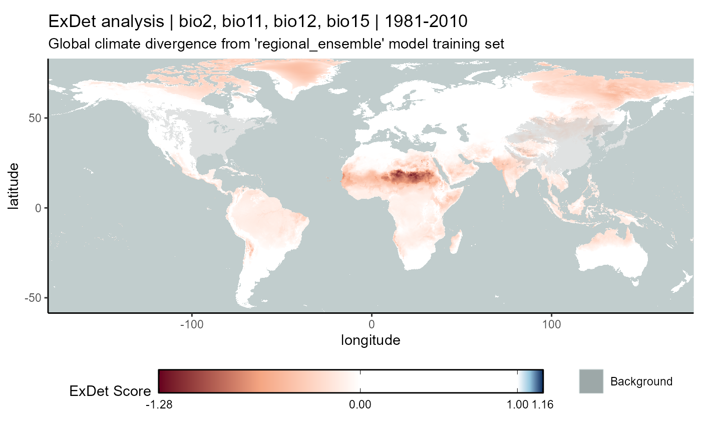

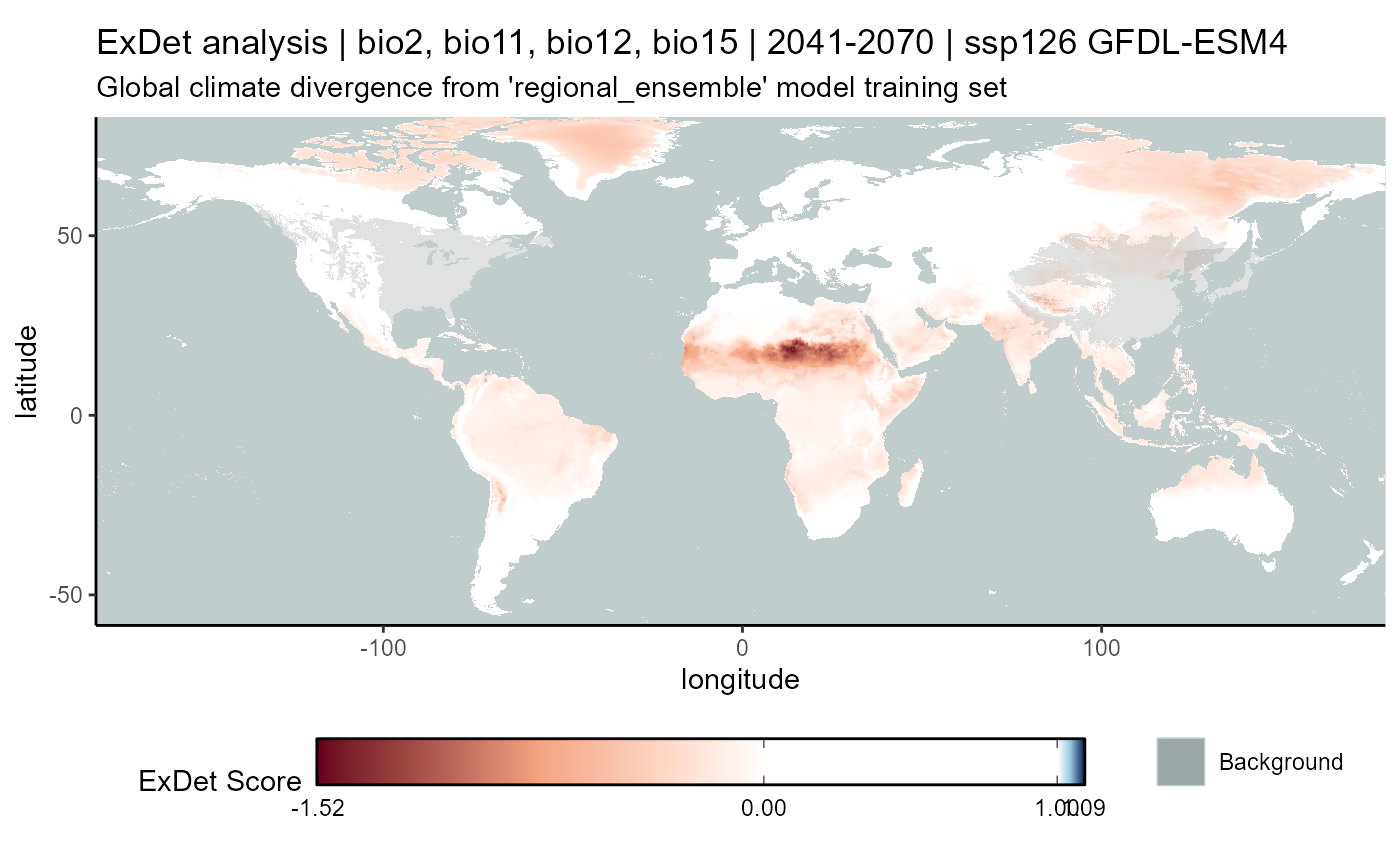
# save plot
ggsave(
  exdet_regional_ensemble_hist_plot, 
  filename = file.path(here::here(), "vignette-outputs", "figures", "ExDet_slf_regional_ensemble_v1_background_projGlobe_1981-2010.jpg"),
  height = 8, 
  width = 12,
  device = jpeg,
  dpi = "retina"
  )

ssp126

# CMIP6
exdet_126_mean <- terra::app(
  x = exdet_126_stack2,
  fun = "mean",
  filename = file.path(
    mypath, "models", "slf_regional_ensemble_v1", "ExDet_slf_regional_ensemble_v1_background_projGlobe_2041-2070_GFDL_ssp126.asc"
    ),
  filetype = "AAIGrid",
  overwrite = FALSE
)

ssp370

# CMIP6
exdet_370_mean <- terra::app(
  x = exdet_370_stack2,
  fun = "mean",
  filename = file.path(
    mypath, "models", "slf_regional_ensemble_v1", "ExDet_slf_regional_ensemble_v1_background_projGlobe_2041-2070_GFDL_ssp370.asc"
    ),
  filetype = "AAIGrid",
  overwrite = FALSE
)

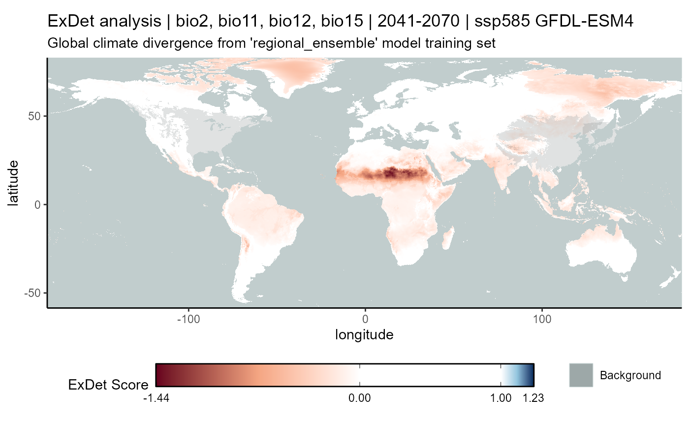
ssp585

# CMIP6
exdet_585_mean <- terra::app(
  x = exdet_585_stack2,
  fun = "mean",
  filename = file.path(
    mypath, "models", "slf_regional_ensemble_v1", "ExDet_slf_regional_ensemble_v1_background_projGlobe_2041-2070_GFDL_ssp585.asc"
    ),
  filetype = "AAIGrid",
  overwrite = FALSE
)

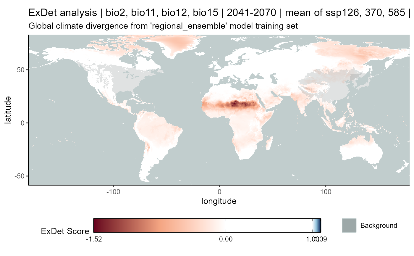
ssp mean

exdet_ssp_mean_stack <- c(exdet_126_mean, exdet_370_mean, exdet_585_mean)

# CMIP6
exdet_ssp_mean <- terra::app(
  x = exdet_ssp_mean_stack,
  fun = "mean",
  filename = file.path(
    mypath, "models", "slf_regional_ensemble_v1", "ExDet_slf_regional_ensemble_v1_background_projGlobe_2041-2070_GFDL_ssp_mean.asc"
    ),
  filetype = "AAIGrid",
  overwrite = FALSE
)

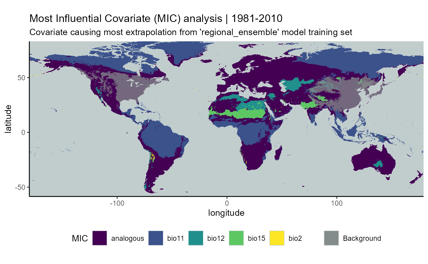
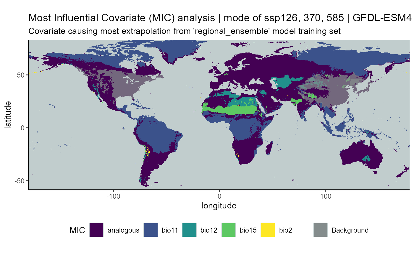
5.2 MIC

I will also ensemble the MIC maps. These will be combined according to the mode (the most common value of the cell) among the 3 rasters.

map_style_MIC <- list(
  theme_classic(),
  theme(legend.position = "bottom",
        panel.background = element_rect(fill = "azure3",
                                        colour = "azure3")
  ),
  scale_x_continuous(expand = c(0, 0)),
  scale_y_continuous(expand = c(0, 0)),
  labs(
    x = "longitude",
    y = "latitude"
  ),
  coord_equal()
)

# color scheme taken from: https://colorbrewer2.org/?type=diverging&scheme=RdBu&n=11

prepare files

mic_regional_native <- terra::rast(
  x = file.path(mypath, "models", "slf_regional_native_v3", "mic_slf_regional_native_v3_background_projGlobe.tif")
)

mic_regional_invaded <- terra::rast(
  x = file.path(mypath, "models", "slf_regional_invaded_v7", "mic_slf_regional_invaded_v7_background_projGlobe.tif")
)

mic_regional_invaded_asian <- terra::rast(
  x = file.path(mypath, "models", "slf_regional_invaded_asian_v2", "mic_slf_regional_invaded_asian_v2_background_projGlobe.tif")
)

# ssp 126
mic_regional_native_126 <- terra::rast(
  x = file.path(mypath, "models", "slf_regional_native_v3", "mic_slf_regional_native_v3_background_projGlobe_2041-2070_ssp126_GFDL.tif")
)
mic_regional_invaded_126 <- terra::rast(
  x = file.path(mypath, "models", "slf_regional_invaded_v7", "mic_slf_regional_invaded_v7_background_projGlobe_2041-2070_ssp126_GFDL.tif")
)
mic_regional_invaded_asian_126 <- terra::rast(
  x = file.path(mypath, "models", "slf_regional_invaded_asian_v2", "mic_slf_regional_invaded_asian_v2_background_projGlobe_2041-2070_ssp126_GFDL.tif")
)

# ssp 370
mic_regional_native_370 <- terra::rast(
  x = file.path(mypath, "models", "slf_regional_native_v3", "mic_slf_regional_native_v3_background_projGlobe_2041-2070_ssp370_GFDL.tif")
)
mic_regional_invaded_370 <- terra::rast(
  x = file.path(mypath, "models", "slf_regional_invaded_v7", "mic_slf_regional_invaded_v7_background_projGlobe_2041-2070_ssp370_GFDL.tif")
)
mic_regional_invaded_asian_370 <- terra::rast(
  x = file.path(mypath, "models", "slf_regional_invaded_asian_v2", "mic_slf_regional_invaded_asian_v2_background_projGlobe_2041-2070_ssp370_GFDL.tif")
)

# ssp 585
mic_regional_native_585 <- terra::rast(
  x = file.path(mypath, "models", "slf_regional_native_v3", "mic_slf_regional_native_v3_background_projGlobe_2041-2070_ssp585_GFDL.tif")
)
mic_regional_invaded_585 <- terra::rast(
  x = file.path(mypath, "models", "slf_regional_invaded_v7", "mic_slf_regional_invaded_v7_background_projGlobe_2041-2070_ssp585_GFDL.tif")
)
mic_regional_invaded_asian_585 <- terra::rast(
  x = file.path(mypath, "models", "slf_regional_invaded_asian_v2", "mic_slf_regional_invaded_asian_v2_background_projGlobe_2041-2070_ssp585_GFDL.tif")
)

# historical
mic_hist_stack2 <- c(mic_regional_native, mic_regional_invaded, mic_regional_invaded_asian)
# CMIP6
mic_126_stack2 <- c(mic_regional_native_126, mic_regional_invaded_126, mic_regional_invaded_asian_126)
mic_370_stack2 <- c(mic_regional_native_370, mic_regional_invaded_370, mic_regional_invaded_asian_370)
mic_585_stack2 <- c(mic_regional_native_585, mic_regional_invaded_585, mic_regional_invaded_asian_585)

historical

# historical
mic_hist_mean <- terra::app(
  x = mic_hist_stack2,
  fun = "modal",
  filename = file.path(mypath, "models", "slf_regional_ensemble_v1", "mic_slf_regional_ensemble_v1_background_projGlobe_1981-2010.asc"),
  filetype = "AAIGrid",
  overwrite = FALSE
)

ssp mode

mic_ssp_mode_stack <- c(mic_126_mean, mic_370_mean, mic_585_mean)

# CMIP6
mic_ssp_mode <- terra::app(
  x = mic_ssp_mode_stack,
  fun = "modal",
  filename = file.path(
    mypath, "models", "slf_regional_ensemble_v1", "mic_slf_regional_ensemble_v1_background_projGlobe_2041-2070_GFDL_ssp_mode.asc"
    ),
  filetype = "AAIGrid",
  overwrite = FALSE
)

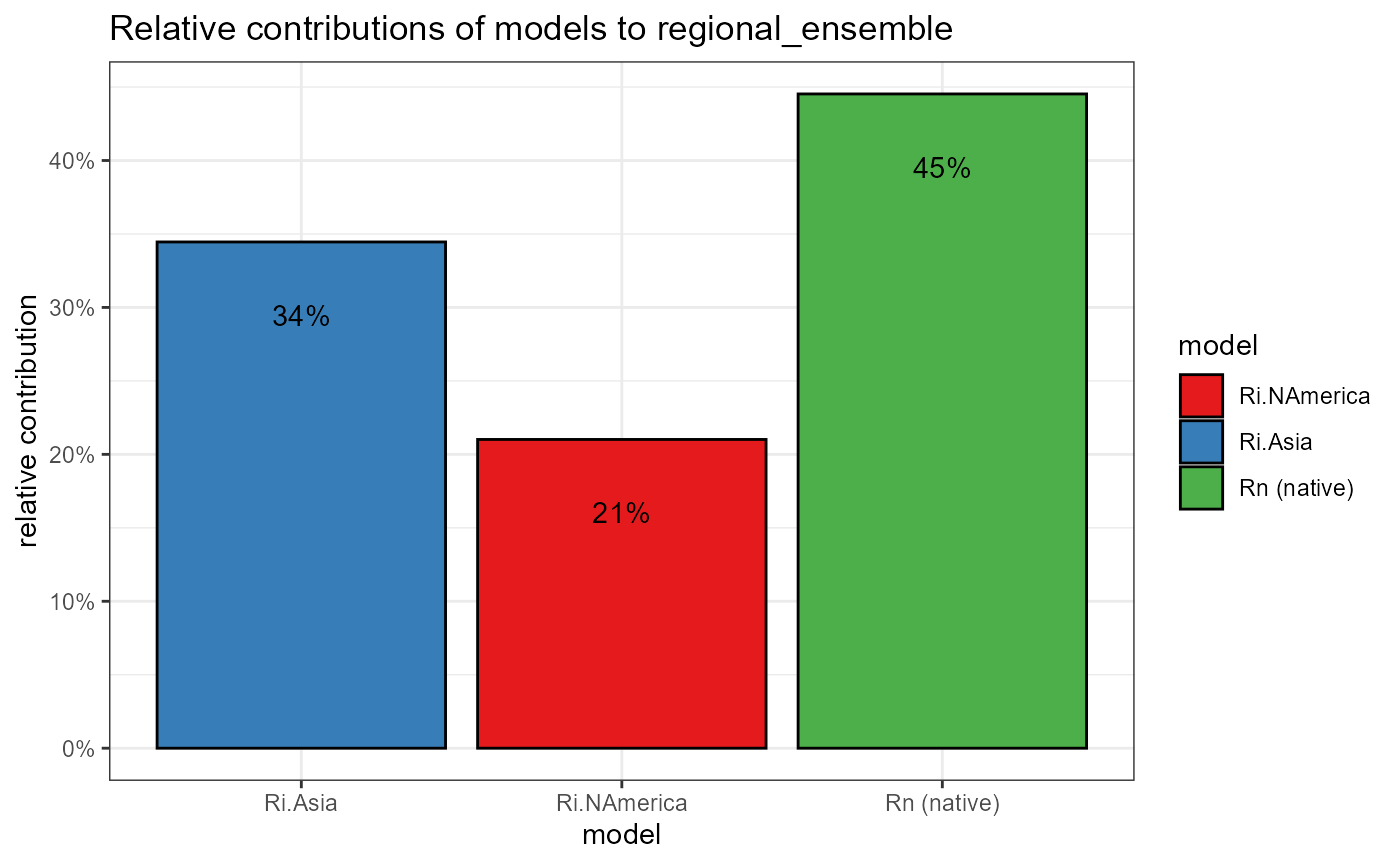
6. plot- Relative weights percent cont

This bar chart will show the relative weights of each of the three regional models as a percent contribution to the total ensemble. I will take the relative weights from each exdet raster, normalize them and plot those weights.

# native
ensemble_weight_regional_native_hist <- terra::rast(file.path(mypath, "models", "slf_regional_ensemble_v1", "ensemble_weights_slf_regional_native_v3.tif"))
# invaded
ensemble_weight_regional_invaded_hist <- terra::rast(file.path(mypath, "models", "slf_regional_ensemble_v1", "ensemble_weights_slf_regional_invaded_v7.tif"))
# invaded_asian
ensemble_weight_regional_invaded_asian_hist <- terra::rast(file.path(mypath, "models", "slf_regional_ensemble_v1", "ensemble_weights_slf_regional_invaded_asian_v2.tif"))

# stack
ensemble_weights_stack <- c(ensemble_weight_regional_native_hist, ensemble_weight_regional_invaded_hist, ensemble_weight_regional_invaded_asian_hist)

# take mean of weights
relative_weights <- c(
  regional_native = mean(values(ensemble_weights_stack[[1]]), na.rm = TRUE),
  regional_invaded = mean(values(ensemble_weights_stack[[2]]), na.rm = TRUE),
  regional_invaded_asian = mean(values(ensemble_weights_stack[[3]]), na.rm = TRUE)
) %>%
  abs() # absolute value 

# sum the weights
relative_weights_sum <- sum(relative_weights)

# normalize weights to sum to 1
relative_weights_prop <- relative_weights / relative_weights_sum %>%
  as.vector() 

# change names of weights
names(relative_weights_prop) <- c("Rn (native)", "Ri.NAmerica", "Ri.Asia")


# plotting colors
ensemble_colors <- c(
  "Ri.NAmerica" =  "#e41a1c",
  "Ri.ASia" = "#377eb8",
  "Rn (native)" = "#4daf4a"
)

Now that we have created an ensembled prediction for our regional-scale models, we can compare them with the global model predictions and explore the suitability for SLF under climate change using suitability maps, point-wise predictions, quadrant plots, variable response curves and others.

References

Araújo, M. B., & New, M. (2007). Ensemble forecasting of species distributions. Trends in Ecology & Evolution, 22(1), 42–47. https://doi.org/10.1016/j.tree.2006.09.010
Elith, J., Kearney, M., & Phillips, S. (2010). The art of modelling range-shifting species. Methods in Ecology and Evolution, 1(4), 330–342. https://doi.org/10.1111/j.2041-210X.2010.00036.x
Mesgaran, M. B., Cousens, R. D., & Webber, B. L. (2014). Here be dragons: A tool for quantifying novelty due to covariate range and correlation change when projecting species distribution models. Diversity and Distributions, 20(10), 1147–1159. https://doi.org/10.1111/ddi.12209

Samuel M. Owens1

2024-08-09

Overview

Setup

Plotting

1. Import datasets

1.1 MaxEnt Predictions

1.2 AUC values

1.3 ExDet rasters

2. Edit import datasets

2.1 Stack rasters

2.2 Preparatory raster edits

3. Ensemble rasters

3.1 Format ExDet rasters into weighting factor

historical

3.2 Weight Models using Test AUC

historical

3.3 Apply weighting factor to models

4. Ensemble thresholds

4.1 Import data

ExDet rasters

4.2 Pred rasters

thresh values

4.3 Create weight for thresh

MTSS

MTP

4.4 Combine in table and export

5. Ensemble ExDet / MIC maps

5.1 ExDet

prepare files

historical

ssp126

ssp370

ssp585

ssp mean

5.2 MIC

prepare files

historical

ssp mode

6. plot- Relative weights percent cont

References

Samuel M. Owens¹