SLF occurrence records: GBIF, lydemapR, literature
Samuel M. Owens1
2025-07-04
Source:vignettes/030_retrieve_occurrence_records.Rmd
030_retrieve_occurrence_records.RmdOverview
In the last vignette, we downloaded bioclimatic rasters from CHELSA and harmonized them to a standard format, including a the resolution, origin and extent.
This vignette will provide instructions to retrieve Lycorma
delicatula (SLF) presence records for the future creation of MaxEnt
models. MaxEnt is a presence-only modeling software, and so it does not
require recorded absence data to predict the suitable area for SLF. Four
categories of data sources will be used in this analysis: GBIF (Global Biodiversity Information
Facility), lydemapR,
various pieces of peer-reviewed literature, and natural history notes.
These data will then be tidied, spatially thinned and compiled into a
single .rds file of SLF presence records that can be loaded
into MaxEnt.
The first step will be to retrieve data from GBIF and
lydemapR. GBIF is an open-access platform for
biodiversity data that gathers from various databases and citizen
science platforms. Data from this source represents globally distributed
presences of SLF. The lyde() function within the
Lydemapr package gives access to nearly one million SLF
presence records within the United States, largely obtained from
biological field surveys by various state and federal departments of
agriculture.
These data will need to be cleaned and tidied during this step. To get to this tidy dataset, the data will be checked for inconsistent and false records. The data will also be spatially thinned so that points are no less than 10km (the resolution of the climate data, 5 arcminutes) to eliminate the effects of sampling bias.
The second step will be to combine these records with data gathered from peer-reviewed literature and from natural history notes. A majority of these records are from established populations of SLF within China, South Korea and southeast Asia. These records are especially important because China and southeast Asia represent the native range for SLF, and there is very little data on the extent of its native range. These records are also important because MaxEnt correlates presence records with the local climate; thus, if there is very little characterization of the native range for this species, it is unlikely that models for SLF will make realistic predictions for its potential niche elsewhere.
The final step of this analysis will be to organize the different
datasets into a single .rds file that can be loaded into
MaxEnt. MaxEnt requires that input datasets contain only 3 columns, in
this order: species (the scientific name of the species),
x (longitude), and y (latitude). Lastly, the
data will go through a second round of spatial thinning now that the
datasets have been joined.
Setup
First, I will load in the necessary packages.
# general tools
library(tidyverse)  #data manipulation
library(here) #making directory pathways easier on different instances
# here() is set at the root folder of this package
library(devtools) # installing packages not from CRAN

# species occurrence data
library(lydemapr) # field survey data for SLF
library(rgbif) #query gbif and format as a dataframe
library(GeoThinneR) # spatial thinning of species occurrences
library(CoordinateCleaner) # tidying of points

# shapefile data
library(rnaturalearth)
library(rnaturalearthdata)
library(rnaturalearthhires)

# spatial
library(terra)

# aesthetics
library(patchwork) #nice plots
library(knitr) # nice rmd tables
Note: I will be setting the global options of this
document so that only certain code chunks are rendered in the final
.html file. I will set the eval = FALSE so that none of the
code is re-run (preventing files from being overwritten during knitting)
and will simply overwrite this in chunks with plots.
I will also download a world map for plotting the data I download
from GBIF and lydemapR. I will use the rnaturalearth
package to download a world map at a scale of 10m.
# check which types of data are available
# these are in the rnaturalearth package
data(df_layers_cultural)
# I will use states_provinces

# get metadata
ne_metadata <- rnaturalearth::ne_find_vector_data(
  scale = 10,
  category = "cultural",
  getmeta = TRUE
) %>%
  dplyr::filter(layer == "admin_0_countries")
# URL to open metadata
utils::browseURL(ne_metadata[, 3])

# if the file isnt already downloaded, download it
if (!file.exists(file.path(here::here(), "data-raw", "ne_countries", "ne_10m_admin_0_countries.shp"))) {

  countries_sf <- rnaturalearth::ne_download(
    scale = 10, # highest resolution
    type = "admin_0_countries", # states and provinces
    category = "cultural",
    destdir = file.path(here::here(), "data-raw", "ne_countries"),
    load = TRUE, # load into environment
    returnclass = "sf" # shapefile
  )

  # else, just import
  } else {

    countries_sf <- sf::read_sf(dsn = file.path(here::here(), "data-raw", "ne_countries", "ne_10m_admin_0_countries.shp"))

  }
Most of this compendium and its functions are built on the
tidyverse language. The here package starts
file pathing from the root folder of my scari package,
allowing easier sharing. The rgbif package will be used to
query records from GBIF, while the lydemapr
package will be used to retrieve field survey data in the United States.
GeoThinneR makes for easy spatial thinning of points and
can employ a grid-based algorithm, so I will use this package.
Validation points- globally important viticultural regions
First, I will visualize the points we will use to validate our future MaxEnt models. These were retrieved by Huron et al, 2022 and represent 1,074 of the most important global viticultural regions. I will also create a transformed version for use with the Behrmann CRS (ESRI:54017).
map_style <- list(
  xlab("UTM Easting"),
  ylab("UTM Northing"),
  theme_classic(),
  theme(legend.position = "bottom",
        panel.background = element_rect(fill = "lightblue2",
                                        colour = "lightblue2")
        ),
  scale_x_continuous(expand = c(0, 0)),
  scale_y_continuous(expand = c(0, 0)),
  viridis::scale_fill_viridis(option = "D"),
  coord_equal()
)
mypath <- file.path(here::here() %>%
                     dirname(),
                   "maxent/historical_climate_rasters/chelsa2.1_30arcsec/v1_maxent_10km")

# background layer
global_bio2_df <- terra::rast(x = file.path(mypath, "bio2_1981-2010_global.asc")) %>%
  terra::as.data.frame(., xy = TRUE)


# load wineries
load(file.path(here::here(), "data-raw", "wineries.rda"))

IVR_locations <- wineries
# I need to transform this dataset to the correct crs
IVR_locations_sv <- terra::vect(IVR_locations, geom = c("x", "y"), crs = "EPSG:4326") %>%
    terra::project(y = "ESRI:54017") %>% # convert to UTM 33N
# convert to geom, which gets coordinates of a spatVector
    terra::geom()
# convert back to data frame
IVR_locations_UTM <- terra::as.data.frame(IVR_locations_sv) %>%
    dplyr::select(-c(geom, part, hole)) %>%
    dplyr::rename("x_utm" = "x", "y_utm" = "y")

# bind OG data
IVR_locations_UTM <- cbind(IVR_locations_UTM, IVR_locations) %>%
  dplyr::select(-c(x, y)) %>%
  dplyr::rename("x" = "x_utm", "y" = "y_utm")

# save transformation for future use
readr::write_rds(x = IVR_locations_UTM, file = file.path(here::here(), "data", "wineries_esri54017.rds"))
IVR_points_plot <- ggplot() +
    geom_raster(data = global_bio2_df, aes(x = x, y = y), fill = "azure1") +
    geom_point(data = IVR_locations_UTM, aes(x = x, y = y), fill = "purple3", shape = 21, size = 1, stroke = 0.3) +
    ggtitle("globally important viticultural regions") +
    map_style +
    theme(
      legend.position = "none",
      axis.title = element_blank(),
      axis.text = element_blank(),
      axis.ticks = element_blank()
) 1. Retrieve data from GBIF and lydemapR and tidy
1.1- GBIF via rgbif
I will begin by retrieving the GBIF taxonomic ID for Lycorma delicatula.
slf_id <- rgbif::occ_search(scientificName = "Lycorma delicatula")[["data"]]

slf_id <- slf_id %>%
  dplyr::select(taxonKey) %>%
  dplyr::slice_head() %>%
  as.character()
I will also perform a few operations specific to rgbif. I will need to enter my user credentials for gbif; to keep these private, I will edit the .Renviron and call them from there. Once this chunk is run and the .Renviron pops up, enter your username, password and email credentials in the following format on lines 1-3:
- GBIF_USER=” ”
- GBIF_PWD=” ”
- GBIF_EMAIL=” ”
Save and close the document.
I will also retrieve a list of country abbreviations to tailor the download. I will be excluding countries in North America (USA, Mexico, Canada) and Taiwan. Lin and Liao did a comprehensive survey for SLF in Taiwan to validate SLF presence records in online repositories and found that these records were likely false (Lin and Liao, 2024).
# edit R environment for user credentials
usethis::edit_r_environ()

# get list of countries
rgbif::enumeration_country(curlopts = list())
Retrieve and save records
The retrieved ID is 5157899. This matches the ID for the SLF repository on GBIF.
Next, retrieve GBIF records using
occ_download(). I will be editing the following GBIF
constraints:
- hasCoordinate: limit records to only those with coordinate data
- year: we will retrieve records between 1981 and 2023. 1981 was chosen as the earliest date because it corresponds with the earliest climate data available.
- occurrenceStatus: set to only presences, because absence data is not needed
- basisOfRecord: here we include everything except fossil records, to ensure that records are within the target time period.
- hasGeospatialIssue: exclude any records with an issue in the coordinate data
- country: the country of the record
# initiate download
slf_gbif <- rgbif::occ_download(
  # general formatting
  type = "and",
  format = "SIMPLE_CSV",
  # inclusion rules
  pred("taxonKey", slf_id), # search by ID, not species name
  pred("hasCoordinate", TRUE),
  pred("hasGeospatialIssue", FALSE),
  pred("occurrenceStatus", "PRESENT"),
  pred_gte("year", 1981), # records from 1981 onwards
  # exclusion rules
  pred_not(pred_in("basisOfRecord", "FOSSIL_SPECIMEN")), # exclude fossil records
  pred_not(pred_in("country", c("US", "MX", "CA"))), # exclude USA, Canada and mexico
  pred_not(pred_in("country", c("TW"))) # exclude Taiwan
)

# be sure to open slf_gbif and retrieve the download key

# check on download status using key
rgbif::occ_download_wait('0103080-250525065834625')
The data have been pulled to the gbif server, but now we must download the data and edit it in a number of ways.
First, I will import the dataset to my working directory. I will also
retrieve the data citation for this download. I will rename the raw
download file. Finally, I will subset the desired columns and save them
as a separate .csv for use in tidying. The raw query and the raw
coordinates will be saved to the data-raw folder. I will
read in the coordinate data saved there afterwards to prepare for data
tidying.
# download the data as a zip to PC
slf_gbif_download <- rgbif::occ_download_get(
  key = '0103080-250525065834625',
  path = file.path(here::here(), "data-raw"),
  # overwrite = TRUE
  ) %>%
  rgbif::occ_download_import()


# .zip file
# unzip
utils::unzip(
  zipfile = file.path(here::here(), "data-raw", "0103080-250525065834625.zip"),
  exdir =  file.path(here::here(), "data-raw")
  )
# rename .csv file
file.rename(
  from = file.path(here::here(), "data-raw", "0103080-250525065834625.csv"),
  to = file.path(here::here(), "data-raw", paste0("slf_gbif_raw_query_", format(Sys.Date(), "%Y-%m-%d"), ".csv"))
  )
# delete original zip
file.remove(file.path(here::here(), "data-raw", "0103080-250525065834625.zip"))


# simplify download into more useable .csv
slf_gbif_download_simple <- slf_gbif_download %>%
  mutate(prov = "gbif") %>%
  dplyr::select(c("species", "decimalLongitude", "decimalLatitude", "countryCode", "prov", "year", "gbifID")) %>% # select desired columns
  # rename for consistency with rest of vignette
  rename("name" = "species",
         "longitude" = "decimalLongitude",
         "latitude" = "decimalLatitude",
         "key" = "gbifID"
  )

# save .csv both outputs for use
write_csv(x = slf_gbif_download_simple,
          file = file.path(here::here(), "data-raw", paste0("slf_gbif_raw_coords_", format(Sys.Date(), "%Y-%m-%d"), ".csv"))
)

write_csv(x = slf_gbif_download_simple_UTM,
          file = file.path(here::here(), "data-raw", paste0("slf_gbif_raw_coords_", format(Sys.Date(), "%Y-%m-%d"), "_esri54017.csv"))
)
rgbif::gbif_citation('0103080-250525065834625')Here is the data citation: “GBIF Occurrence Download https://doi.org/10.15468/dl.h4zzpe Accessed from R via rgbif (https://github.com/ropensci/rgbif) on 2025-07-07”
There are 2154 total records from GBIF. Datasets = NULL
Coordinate veracity
First, we want to check the coordinate veracity using the
CoordinateCleaner package. We will be more picky and apply
more tests to the GBIF data points than those from the other datasets
because they are usually less accurate than field survey data.
- valid and likely coordinates
- points set to the centroid of a country or province
- coordinates that fall into the ocean
- duplicates
- points with equal lat / lon
- points near the GBIF HQ
- points near biodiv institutions
- points near whole lat / lon numbers
# read in data
slf_gbif_coords1 <- readr::read_csv(file = file.path(here::here(), "data-raw", "slf_gbif_raw_coords_2025-07-07.csv"))

# set random seed
set.seed(999)

# coordinate cleaner
slf_gbif_report <- CoordinateCleaner::clean_coordinates(
  x = slf_gbif_coords1,
  lon = "longitude",
  lat = "latitude",
  species = "name",
  tests = c("centroids", "duplicates", "equal", "gbif", "institutions", "seas", "zeros"),
  # test details
  seas_scale = 110,
  centroids_detail = "both",
  verbose = TRUE
) %>%
  as.data.frame()
It seems like the most records were removed for duplicate records, followed by for records flagged as being in the ocean or other bodies of water. We also did find a few records that were attributed to biodiversity institutions and country / province centroids.
Next, I will filter out problematic points and ensure the species naming is consistent.
# remove flagged records
slf_gbif_coords1 <- slf_gbif_report %>%
  dplyr::filter(.summary == TRUE) # FALSE records are potentially problematic

# check species name
unique(slf_gbif_coords1$name)

# there is only one naming convention
This process left 1913 of 2154 total points.
Next, we will use GeoThinneR::thin_points to spatially
thin the occurrence data. The GeoThinneR package was chosen
to perform the initial thinning because it preserves non-coordinate data
in its output. So, we can save a spatially thinned version of the data
with other information (such as unique keys or dates) that might be
useful later.
In GeoThinneR::thin_points(), The data will be rarefied
to 10km over 10 passes. This will be done once more on the final
dataset. Spatial thinning should reduce autocorrelation and sampling
bias. I have programmed this function to rarefy at 10km, which is the
current resolution of the climate data we used from
CHELSA.GeoThinneR has a grid
function that will thin species data based on a predetermined raster, so
we will use the CHELSA rasters we tidied and aggregated in
the last vignette. These rasters originally came at a resolution of 30
arc-seconds (roughly 1km at the equator) but we aggregated them at 10km
by taking the mean value per cell. We will also perform this process
separately for different countries. I am using a special reference layer
I created that is identical to the rasters that will be used for the
MaxEnt models, except that it is projected into the
EPSG:4326 coordinate reference system (CRS), instead of the
ESRI:54107 crs.
slf_gbif_coords2 <- GeoThinneR::thin_points(
  data = slf_gbif_coords1,
  long_col = "longitude",
  lat_col = "latitude",
  method = "grid", # use a grid based thinning method
  raster_obj = geothinner_raster, # the aggregated raster to use
  group_col = "countryCode", # additionally thin separately based on country
  trials = 10, # number of passes
  seed = 997, # set reproducible seed
  verbose = TRUE
  )

View(slf_gbif_coords2[[1]])

# get rid of unnecessary columns used for thinning
slf_gbif_coords2 <- slf_gbif_coords2[[1]] %>% dplyr::select(name:key)
Spatial thinning left 656 of 1323 total records. It left 505 of 1,489
observations with the old Humboldt package.
We will save the results of the cleaning we just performed so they can be referenced or called later in our analysis. Later in this vignette, we will be combining these records with those from other data sources into a final dataset that is prepared for MaxEnt.
1.2- LydemapR
Retrieve and save lydemapR records
Next, we will retrieve data from the lydemapR package and save it as
a .csv. I will repeat the spatial thinning and cleaning
process outlined above.
slf_lyde <- lydemapr::lyde

write_csv(x = slf_lyde,
          file = file.path(here::here(), "data-raw", paste0("slf_lyde_raw_coords_", format(Sys.Date(), "%Y-%m-%d"), ".csv")))
The next chunk is an import from an unpublished version of the lydemapr dataset. This version will be published on the package soon, but for now we will use this . This file was named “slf_lyde_raw_coords_2024-07-29.csv” for consistency with previous file naming. It contains about 900,000 published SLF records and includes the years 2022 and 2023.
if (FALSE) {

  slf_lyde_raw <- readr::read_csv(file = file.path(here::here(), "data-raw", "slf_lyde_raw_coords_2025-07-07.csv"))

  # overwrite save original version
  write_csv(x = slf_lyde_raw, file = file.path(here::here(), "data-raw", "slf_lyde_raw_coords_2025-07-07.csv"))

}
The raw dataset is composed of over 658,000 records of SLF in the USA alone. Most of these records are concentrated in the mid-atlantic region where the invasion front is progressing. This dataset will also need a run of spatial thinning. First, we will need to narrow these records to fit our needs. At the time of writing this, I am only interested in records that were collected during field surveys, but this can be tuned to the needs of the analysis. So, I will set the collection method equal to the value of “field_survey/management”. Obviously, I am also interested in presence records only.
Lastly, I will pull records only from areas where SLF have established a population. LydemapR defines an established population as either 2+ adults or the presence of 1 egg mass.
# read in data
slf_lyde <- readr::read_csv(file = file.path(here::here(), "data-raw", "slf_lyde_raw_coords_2025-07-07.csv"))

# unique values for collection method
unique(slf_lyde$collection_method)

slf_lyde1 <- slf_lyde %>%
  dplyr::filter(lyde_present == "TRUE", # only select presences
         collection_method == "field_survey/management", # collection method = "field_survey/management"
         lyde_established == "TRUE") %>% # only select areas records that are from established populations
  # add species column
  dplyr::mutate(species = "Lycorma delicatula")
The data that fit our needs are about 55,000 records total.
Coordinate veracity
Here we will run through the same data cleaning process that we
performed for the GBIF data.
set.seed(996)

# coordinate cleaner
slf_lyde_report <- CoordinateCleaner::clean_coordinates(
  x = slf_lyde1,
  lon = "longitude",
  lat = "latitude",
  species = "species",
  tests = c("centroids", "duplicates", "equal", "gbif", "institutions", "seas", "zeros"),
  # test details
  seas_scale = 110,
  centroids_detail = "both"
) %>%
  as.data.frame()

# remove flagged records
slf_lyde1 <- slf_lyde_report %>%
  dplyr::filter(.summary == TRUE) # FALSE records are potentially problematic
Again, the majority were duplicates, followed by those that fell into bodies of water.
slf_lyde2 <- GeoThinneR::thin_points(
  data = slf_lyde1,
  long_col = "longitude",
  lat_col = "latitude",
  method = "grid", # use a grid based thinning method
  raster_obj = geothinner_raster, # the aggregated raster to use
  trials = 10, # number of passes
  seed = 995, # set reproducible seed
  verbose = TRUE
  )

# get rid of unnecessary columns used for thinning
slf_lyde2 <- slf_lyde2[[1]] %>% dplyr::select(source:species)
Spatial thinning for the lyde dataset left 1386 points
out of the 39,000 points that fit our needs. Previous usage of the
Humboldt package left 366 points out of 39,000.
1.3- Visualize SLF distributions
We want to visualize the difference between the raw coordinates that were pulled from GBIF and the cleaned, spatially thinned version. This is to ensure proper geospatial coverage and the success of the spatial thinning runs.
# raw data
gbif_raw <- readr::read_csv(file = file.path(here::here(), "data-raw", "slf_gbif_raw_coords_2025-07-07.csv"))

# thinned data
gbif_thinned <- readr::read_csv(file = file.path(here::here(), "vignette-outputs", "data-tables", "slf_gbif_cleaned_coords_2025-07-07.csv"))

# plot world map
map_gbif_thinned <- ggplot() +
  # basemap
  geom_sf(data = countries_sf, aes(geometry = geometry), fill = NA, color = "black", lwd = 0.15) +
  geom_point(data = gbif_raw, aes(x = longitude, y = latitude), color = "blue", size = 2) +
  geom_point(data = gbif_thinned, aes(x = longitude, y = latitude), color = "darkorange", shape = 2) +
  coord_sf(xlim = c(-164.5, 163.5), ylim = c(-55, 85)) +
  ggtitle("SLF GBIF records- \n raw (blue) vs thinned (darkorange)") +
  theme(panel.grid.major = element_blank(),
        panel.grid.minor = element_blank(),
        panel.background = element_blank()) +
  theme_bw() +
  theme(axis.title = element_blank())

# plot map of Asia
map_gbif_thinned_Asia <- ggplot() +
  # basemao
  geom_sf(data = countries_sf, aes(geometry = geometry), fill = NA, color = "black", lwd = 0.15) +
  geom_point(data = gbif_raw, aes(x = longitude, y = latitude), color = "blue", size = 2) +
  geom_point(data = gbif_thinned, aes(x = longitude, y = latitude), color = "darkorange", shape = 2) +
  coord_sf(xlim = c(100, 140), ylim = c(20, 50)) +
  ggtitle("SLF GBIF records in Asia-\nraw (blue) vs thinned (darkorange)") +
  theme(panel.grid.major = element_blank(),
        panel.grid.minor = element_blank(),
        panel.background = element_blank()) +
  theme_bw() +
  theme(axis.title = element_blank())

# patchwork display of plots
map_gbif_thinned + map_gbif_thinned_Asia +
  plot_layout(nrow = 2)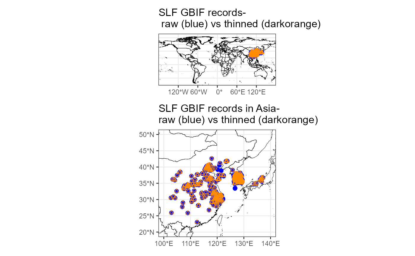
From the mapping, it seems that the spatial thinning reduced the GBIF records, while preserving the same spatial extent. We also zoom in on the invaded range, and indeed every blue point is paired with at least 1 darkorange point. So, our goal was met! We will do the same for the LydemapR data to ensure spatial thinning success.
# raw data
lyde_raw <- readr::read_csv(file = file.path(here::here(), "data-raw", "slf_lyde_raw_coords_2025-07-07.csv"))

# thinned data
lyde_thinned <- readr::read_csv(file = file.path(here::here(), "vignette-outputs", "data-tables", "slf_lyde_cleaned_coords_2025-07-07.csv"))

# ensure data points represent presences
lyde_raw <- lyde_raw %>%
  filter(lyde_present == "TRUE")

# plot map of NAmerica
map_lyde_allRecords <- ggplot() +
  geom_sf(data = countries_sf, aes(geometry = geometry), fill = NA, color = "black", lwd = 0.15) +
  geom_point(data = lyde_raw, aes(x = longitude, y = latitude), color = "blue", size = 2) +
  geom_point(data = lyde_thinned, aes(x = longitude, y = latitude), color = "darkorange", shape = 2) +
  coord_sf(xlim = c(-133.593750, -52.294922), ylim = c(25.085599, 55.304138)) +
  ggtitle("SLF lydemapR records- \nall records (blue)\nvs thinned (darkorange)") +
  theme(panel.grid.major = element_blank(),
        panel.grid.minor = element_blank(),
        panel.background = element_blank()) +
  theme_bw()


# include only established records
lyde_raw1 <- lyde_raw %>%
  filter(lyde_established == "TRUE") %>%
  mutate(species = "Lycorma delicatula")


# plot map including only established records
map_lyde_estab <- ggplot() +
  geom_sf(data = countries_sf, aes(geometry = geometry), fill = NA, color = "black", lwd = 0.15) +
  geom_point(data = lyde_raw1, aes(x = longitude, y = latitude), color = "blue", size = 2) +
  geom_point(data = lyde_thinned, aes(x = longitude, y = latitude), color = "darkorange", shape = 2) +
  coord_sf(xlim = c(-90, -70), ylim = c(35, 45)) +
  ggtitle("SLF lydemapR records- \nall records estab populations (blue)\nvs thinned (darkorange)") +
  theme(panel.grid.major = element_blank(),
        panel.grid.minor = element_blank(),
        panel.background = element_blank()) +
  theme_bw()

# patchwork display of plots
 map_lyde_allRecords + map_lyde_estab +
  plot_layout(nrow = 2)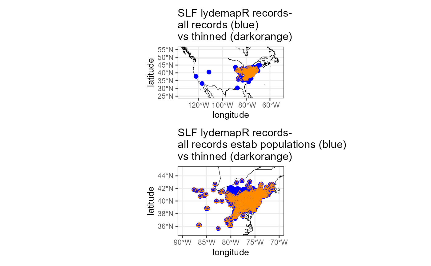
The spatial thinning was successful! However, the first plot does not help us to understand what data were eliminated by the spatial thinning. It would be an issue if we lost spatial extent for removing certain types of data. I believe this is likely due to our preference for records that represent established populations and for excluding regulatory incidents and unconfirmed populations, so I will plot the reduced raw dataset vs our thinned dataset. Indeed, regulatory incidents and unconfirmed populations account for most of the populations that we excluded (we want this).
2. Combine records
2.1- SLF data from published sources
In this step, I will combine the records obtained from GBIF and LydemapR with data taken from the literature. I will begin by loading in records taken from the published literature. There are a total of 165 records from China, southeast Asia, Japan, SK and the USA. Most of these records were obtained from genetic studies and represent samples taken from established populations of SLF. Data is scarce for established populations of SLF within its native range (China and southeast Asia), so these records are especially important. These records were taken from both peer-reviewed literature and natural history notes.
I had to transform many records using a coordinate converted; I used a few sites: - epsg.io: https://epsg.io/transform#s_srs=4326&t_srs=54017&x=NaN&y=NaN - UMinn PCG: https://applications.pgc.umn.edu/convert/
# read in .csv of papers
slf_published_papers <- readr::read_csv(file.path(here::here(), "data-raw", "slf_publishedOccurrenceRecords_papers.csv"))

# kable table

slf_published_papers %>%
  dplyr::select(!Notes) %>%
knitr::kable(format = "pipe")| Author | Year | Spatial Extent of Records | DOI |
|---|---|---|---|
| Du et al | 2021 | China, Japan, SK, USA | 10.1111/eva.13170 |
| Fennah | 1953 | China | NA |
| Han et al | 2008 | SK | 10.1111/j.1748-5967.2008.00188.x |
| Kim et al | 2013 | China, Japan, SK | 10.1016/j.aspen.2013.07.003 |
| Kim et al | 2021 | China, Japan, SK | 10.3390/insects12060539 |
| Manzoor et al | 2021 | China | 10.1111/aab.12674 |
| Nakashita et al | 2022 | China, Japan, SK, USA | 10.1038/s41598-022-05541-z |
| Suzuki | 2023 | Japan | NA |
| Xin et al | 2020 | China | 10.1093/ee/nvaa137 |
| Yang et al | 2015 | China | 10.11865/zs.20150305 |
| Zhang et al | 2019 | China | 10.3390/insects10100312 |
| Kamiyama et al | 2024 | Japan | 10.1002/1438-390X.12203 |
slf_published_papers## # A tibble: 12 × 5
## Author Year `Spatial Extent of Records` DOI Notes
## <chr> <dbl> <chr> <chr> <chr>
## 1 Du et al 2021 China, Japan, SK, USA 10.1111/eva.13170 NA
## 2 Fennah 1953 China NA repr…
## 3 Han et al 2008 SK 10.1111/j.1748-5967.… NA
## 4 Kim et al 2013 China, Japan, SK 10.1016/j.aspen.2013… NA
## 5 Kim et al 2021 China, Japan, SK 10.3390/insects12060… NA
## 6 Manzoor et al 2021 China 10.1111/aab.12674 repr…
## 7 Nakashita et al 2022 China, Japan, SK, USA 10.1038/s41598-022-0… NA
## 8 Suzuki 2023 Japan NA NA
## 9 Xin et al 2020 China 10.1093/ee/nvaa137 NA
## 10 Yang et al 2015 China 10.11865/zs.20150305 repr…
## 11 Zhang et al 2019 China 10.3390/insects10100… NA
## 12 Kamiyama et al 2024 Japan 10.1002/1438-390X.12… NA
slf_published <- readr::read_csv(file.path(here::here(), "data-raw", "slf_publishedOccurrenceRecords_v3.csv"))## Rows: 198 Columns: 11
## ── Column specification ────────────────────────────────────────────────────────
## Delimiter: ","
## chr (8): name, key, country, stateProvince, publishingArticle, accessionNum,...
## dbl (3): longitude, latitude, year
##
## ℹ Use `spec()` to retrieve the full column specification for this data.
## ℹ Specify the column types or set `show_col_types = FALSE` to quiet this message.
# save as .rds before proceeding
write_rds(x = slf_published, file = file.path(here::here(), "data", "slf_publishedOccurrenceRecords_v3.rds"))
map_published_Asia <- ggplot() +
  # basemap
  geom_sf(data = countries_sf, aes(geometry = geometry), fill = NA, color = "black", lwd = 0.15) +
  geom_point(data = slf_published, aes(x = longitude, y = latitude), color = "darkorange") +
  coord_sf(xlim = c(100, 140), ylim = c(10, 45)) +
  ggtitle("SLF data from published sources \n in China") +
  theme(panel.grid.major = element_blank(),
        panel.grid.minor = element_blank(),
        panel.background = element_blank()) +
  theme_bw() +
  theme(axis.title = element_blank())

map_published_NAmerica <- ggplot() +
  # basemap
  geom_sf(data = countries_sf, aes(geometry = geometry), fill = NA, color = "black", lwd = 0.15) +
  geom_point(data = slf_published, aes(x = longitude, y = latitude), color = "darkorange") +
  coord_sf(xlim = c(-133.593750, -52.294922), ylim = c(25.085599, 55.304138)) +
  ggtitle("SLF data from published sources \n in N America") +
  theme(panel.grid.major = element_blank(),
        panel.grid.minor = element_blank(),
        panel.background = element_blank()) +
  theme_bw() +
  theme(axis.title = element_blank())

# bounding box coords found at:
# http://bboxfinder.com/#0.000000,0.000000,0.000000,0.000000

# patchwork
map_published_Asia + map_published_NAmerica +
  plot_layout(nrow = 2)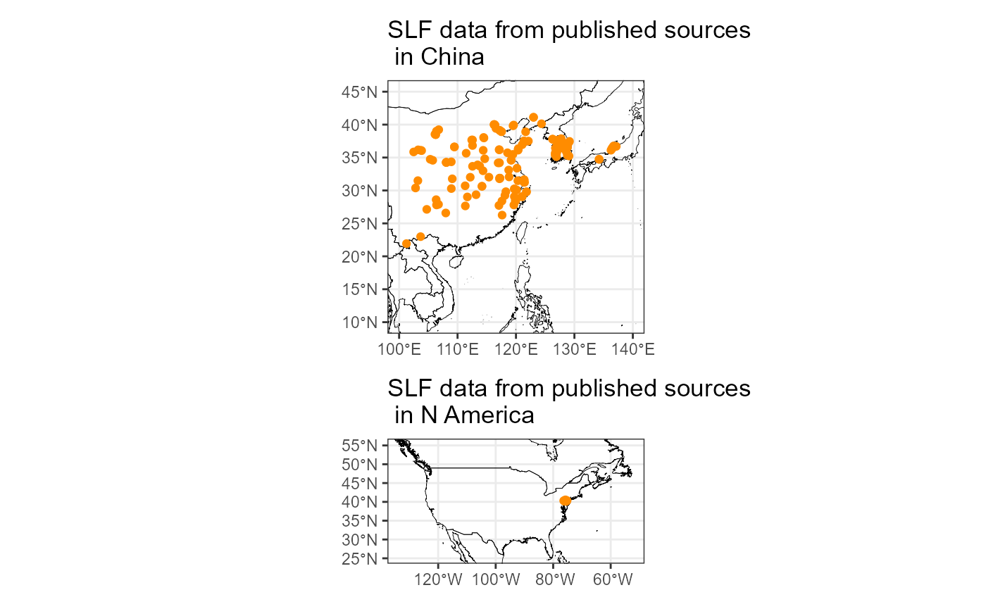
The map above shows that the occurrence data from the literature provide good coverage of the native range that we might not otherwise get.
2.2- Tidy and join datasets
Now, I will load in the cleaned coordinates from GBIF and LydemapR that we produced earlier.
slf_gbif_coords3 <- readr::read_csv(file.path(here::here(), "vignette-outputs", "data-tables", "slf_gbif_cleaned_coords_2025-07-07.csv"))

slf_lyde3 <- readr::read_csv(file.path(here::here(), "vignette-outputs", "data-tables", "slf_lyde_cleaned_coords_2025-07-07.csv"))
First, I will tidy the data for joining. We will keep only the species names, coordinates and unique key ID. We will also add a column that states which data source each point is from.
# tidy gbif data
slf_gbif_coords3 %<>%
  dplyr::select(name:latitude, key, prov) %>%
  rename("data_source" = "prov",
         "species" = "name")

# tidy lyde data
slf_lyde3 %<>%
  dplyr::select(species, longitude, latitude, pointID) %>%
  rename("key" = "pointID") %>%
  mutate(data_source = "lyde")

# published data
slf_published %<>%
  dplyr::select(name:key, publishingArticle) %>%
  rename("species" = "name",
         "data_source" = "publishingArticle")

# the publishing data source column needs to be tidied further. I will take out commas and substitute spaces for underscores
slf_published$data_source <- gsub(pattern = " ", replacement = "_", x = slf_published$data_source)
slf_published$data_source <- gsub(pattern = ",", replacement = "", x = slf_published$data_source)

# Finally, use head() to check coltypes are the same
head(slf_lyde3)
head(slf_gbif_coords3)
head(slf_published)

# we see that the key column in the GBIF dataset is a double, while the key columns in the other 2 are characters. We will change this:
slf_gbif_coords3$key <-  as.character(slf_gbif_coords3$key)

head(slf_gbif_coords3)

# the conversion worked
3. Final Data Tidying
Now the data are in a format that is easier to join. We will join the data and save the cleaned coordinates.
write_csv(x = slf_all_coords, file = file.path(here::here(), "vignette-outputs", "data-tables", "slf_all_coords_2025-07-07.csv"))3.1- Final spatial thinning
The last step of tidying these data is to perform a second round of
spatial thinning. We need to do this again because after joining 3
different datasets together, some of the points may be within 10km of
each other. The data will be rarefied to 10km over 10 passes. This will
be done once more on the final dataset. Spatial thinning should reduce
autocorrelation and sampling bias. Again, we will thin to a minimum of
10km distance between points. We will repeat the process above of using
CoordinateCleaner and GeoThinneR.
Both files will be written to the vignettes-outputs
folder, which holds intermediate data objects that are not the final
versions of the data.
slf_all_coords1 <- GeoThinneR::thin_points(
  data = slf_all_coords,
  long_col = "longitude",
  lat_col = "latitude",
  method = "grid", # use a grid based thinning method
  raster_obj = geothinner_raster, # the aggregated raster to use
  trials = 10, # number of passes
  seed = 995, # set reproducible seed
  verbose = TRUE
  )

slf_all_coords1 <- slf_all_coords1[[1]]
This thinning method left 2131 of 2240 records.
# coordinate cleaner
slf_all_coords_report <- CoordinateCleaner::clean_coordinates(
  x = slf_all_coords1,
  lon = "longitude",
  lat = "latitude",
  species = "species",
  tests = c("centroids", "duplicates", "equal", "gbif", "institutions", "seas", "zeros")
) %>%
  as.data.frame()

# no duplicates!

# remove flagged records
slf_all_coords2 <- slf_all_coords_report %>%
  dplyr::filter(.summary == TRUE) %>% # FALSE records are potentially problematic
  dplyr::select(species:latitude)
This thinning method removed an additional ~40 records, reducing the final number to 2090.
Finally, I will re-run the GeoThinneR method,
additionally using a raw distance metric
slf_all_coords3 <- GeoThinneR::thin_points(
  data = slf_all_coords2,
  long_col = "longitude",
  lat_col = "latitude",
  method = "brute_force",
  #euclidean = TRUE, # use the euclidean distance metric because these coordinates are projected to a lat/long system
  thin_dist = 10,
  seed = 995, # set reproducible seed
  verbose = TRUE
  )

slf_all_coords3 <- slf_all_coords3[[1]]
This method removed a lot of coordinates- reducing the final count from 2040 to 1282 records.
3.2- Save output for MaxEnt
We will finally convert the slf coordinates to the format that will
be used by MaxEnt and save it. That is, the first column “species” must
be the species name, the second column “x” must be the longitude, and
the third column “y” must be the latitude. We will also need to
transform the coordinates to the ESRI:54017 coordinate
reference system (CRS) we used in the previous vignette.
# save EPSG4326 version before transformation
write_csv(x = slf_all_coords3, file = file.path(here::here(), "vignette-outputs", "data-tables", paste0("slf_all_coords_final_2025-07-07_epsg4326.csv")))

# rename columns
slf_all_coords4 <- slf_all_coords3 %>%
  rename("x" = "longitude",
         "y" = "latitude")

# transform CRS of downloaded data
slf_all_coords4 <- terra::vect(slf_all_coords4, geom = c("x", "y"), crs = "EPSG:4326") %>%
    terra::project(y = "ESRI:54017") %>% # convert to UTM 33N
# convert to geom, which gets coordinates of a spatVector
    terra::geom()
# convert back to data frame
slf_all_coords5 <- terra::as.data.frame(slf_all_coords4) %>%
  dplyr::select(-c(geom, part, hole)) %>%
  # join original dataset back for data
  cbind(., slf_all_coords3) %>%
  # remove lat long and other edits
  dplyr::select(-c(longitude, latitude)) %>%
  dplyr::rename(utm_easting = x, utm_northing = y) %>%
  dplyr::relocate(species)
# save
write_csv(x = slf_all_coords5, file = file.path(here::here(), "vignette-outputs", "data-tables", paste0("slf_all_coords_final_2025-07-07.csv")))

# also save as a .rds file
write_rds(slf_all_coords5, file = file.path(here::here(), "data", paste0("slf_all_coords_final_2025-07-07.rds")))
slf_all_coords_df <- readr::read_csv(file = file.path(here::here(), "vignette-outputs", "data-tables", "slf_all_coords_final_2025-07-07_epsg4326.csv"))## Rows: 1282 Columns: 3
## ── Column specification ────────────────────────────────────────────────────────
## Delimiter: ","
## chr (1): species
## dbl (2): longitude, latitude
##
## ℹ Use `spec()` to retrieve the full column specification for this data.
## ℹ Specify the column types or set `show_col_types = FALSE` to quiet this message.
 map_all <- ggplot() +
    # basemap
    geom_sf(data = countries_sf, aes(geometry = geometry), fill = NA, color = "black", lwd = 0.15) +
    geom_point(data = slf_all_coords_df, aes(x = longitude, y = latitude), color = "darkorange", size = 1) +
    coord_sf(xlim = c(-164.5, 163.5), ylim = c(-55, 85)) +
    ggtitle("All SLF presences") +
    theme(panel.grid.major = element_blank(),
          panel.grid.minor = element_blank(),
          panel.background = element_blank()) +
    theme_bw() +
    theme(axis.title = element_blank())

 map_all_NAmerica <- ggplot() +
    # basemap
    geom_sf(data = countries_sf, aes(geometry = geometry), fill = NA, color = "black", lwd = 0.15) +
    geom_point(data = slf_all_coords_df, aes(x = longitude, y = latitude), color = "darkorange", size = 1) +
    coord_sf(xlim = c(-133.593750, -52.294922), ylim = c(25.085599, 55.304138)) +
    ggtitle("SLF presences N America") +
    theme(panel.grid.major = element_blank(),
          panel.grid.minor = element_blank(),
          panel.background = element_blank()) +
    theme_bw() +
    theme(axis.title = element_blank())

  map_all_Asia <- ggplot() +
    # basemap
    geom_sf(data = countries_sf, aes(geometry = geometry), fill = NA, color = "black", lwd = 0.15) +
    geom_point(data = slf_all_coords_df, aes(x = longitude, y = latitude), color = "darkorange", size = 1) +
    coord_sf(xlim = c(68.906250, 152.534180), ylim = c(8.928487, 45.920587)) +
    ggtitle("SLF presences Asia") +
    theme(panel.grid.major = element_blank(),
          panel.grid.minor = element_blank(),
          panel.background = element_blank()) +
    theme_bw() +
    theme(axis.title = element_blank())

# patchwork
map_all_NAmerica + map_all_Asia +
plot_layout(nrow = 2)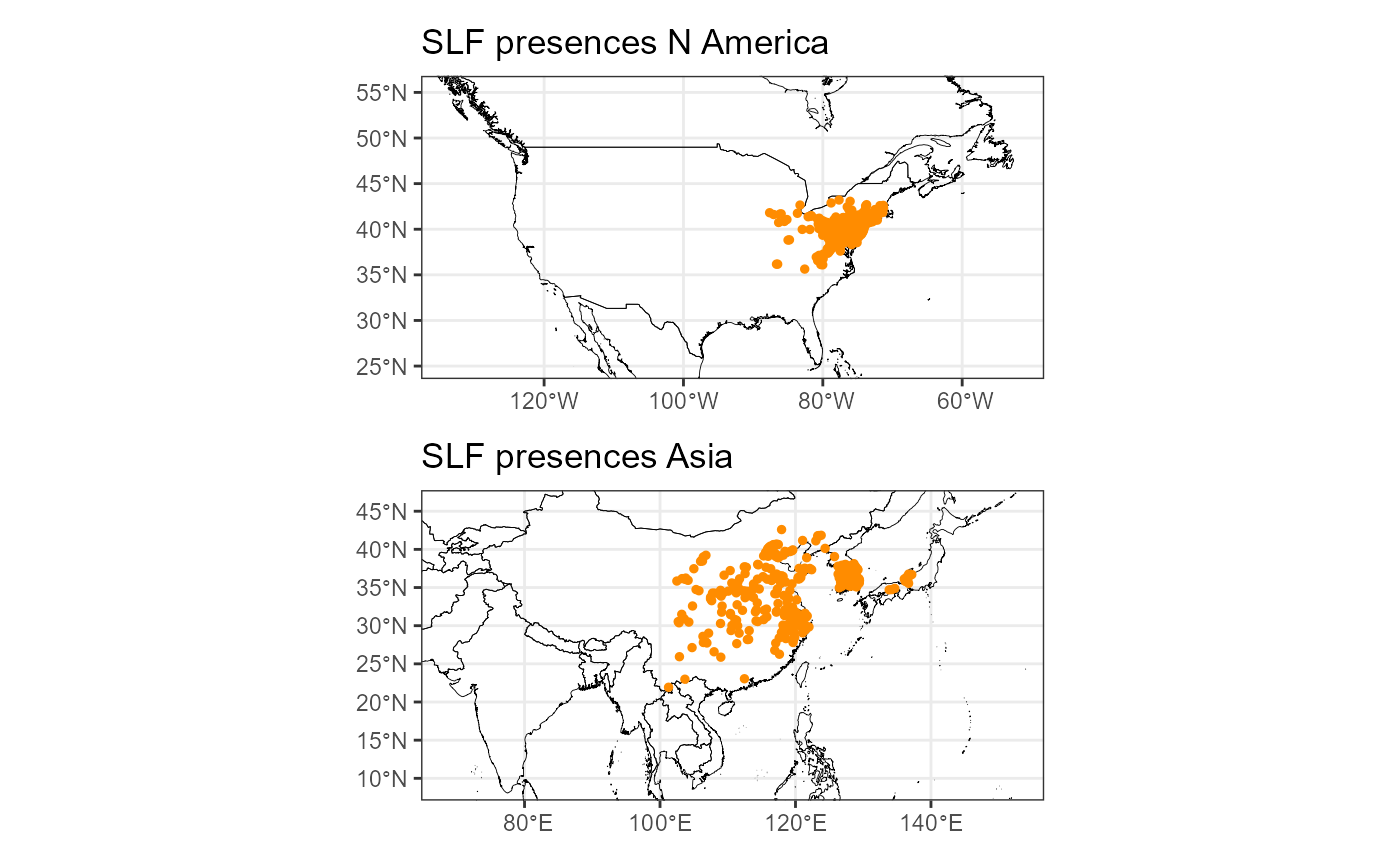
map_all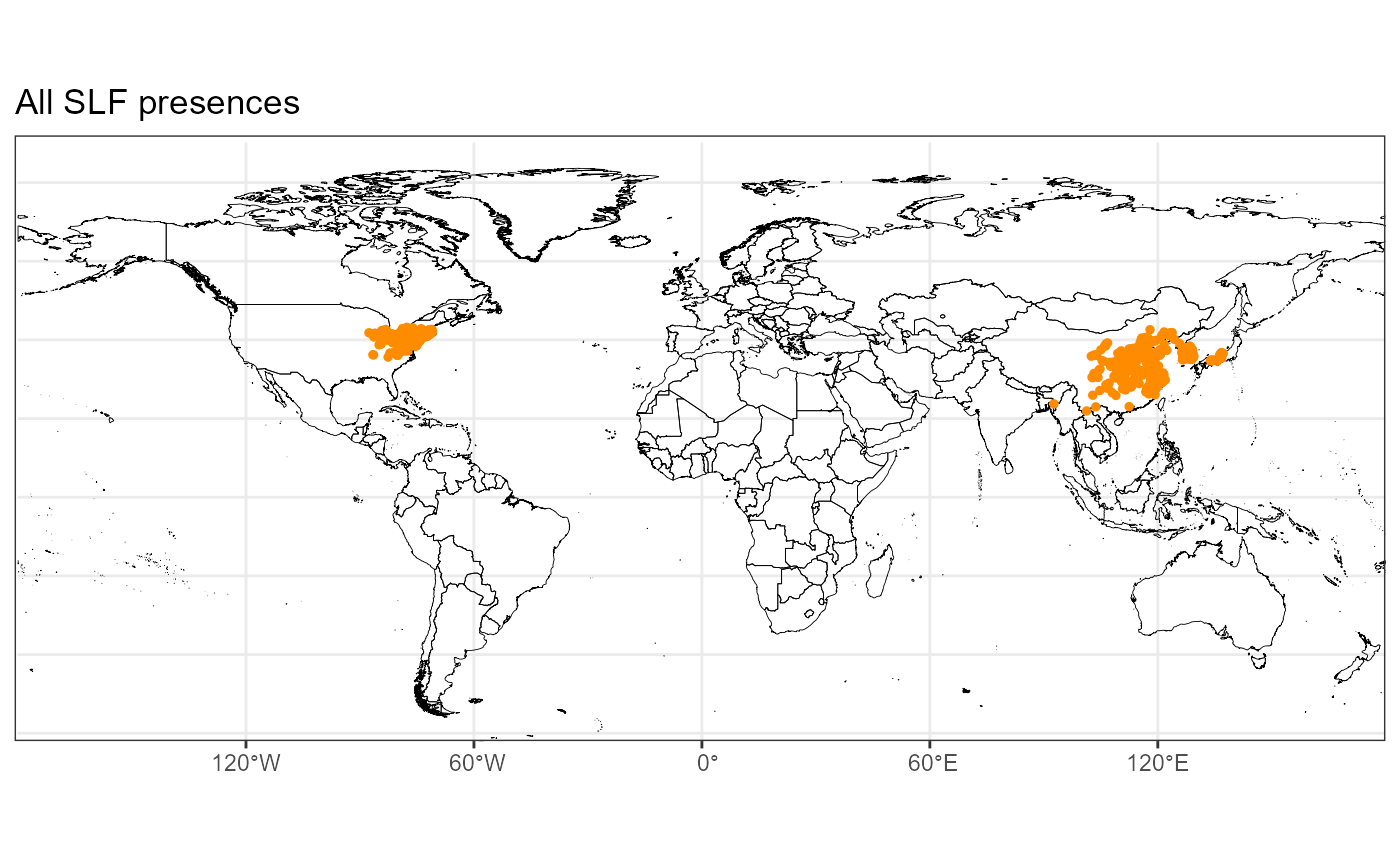
From the map, we can see the final points that were selected. We have a good spread across the native range and better spread than before in the invaded range. This version of the total dataset included newer data from lydemapr, so we now have better coverage in the invaded range. I will also check the number of points in the native vs the invaded range.
SLF_by_longitude <- ggplot(data = slf_all_coords_df) +
  geom_histogram(aes(x = longitude)) +
  ggtitle("count of SLF presence records invaded vs native range") +
  labs(caption = "the longitudinal range between the two dashed lines represents the native range for SLF") +
  xlab("longitude") +
  ylab("count of SLF presences") +
  geom_vline(xintercept = 73.37, linetype = "dashed") +
  geom_vline(xintercept = 124.06, linetype = "dashed") +
  theme_minimal()

SLF_by_longitude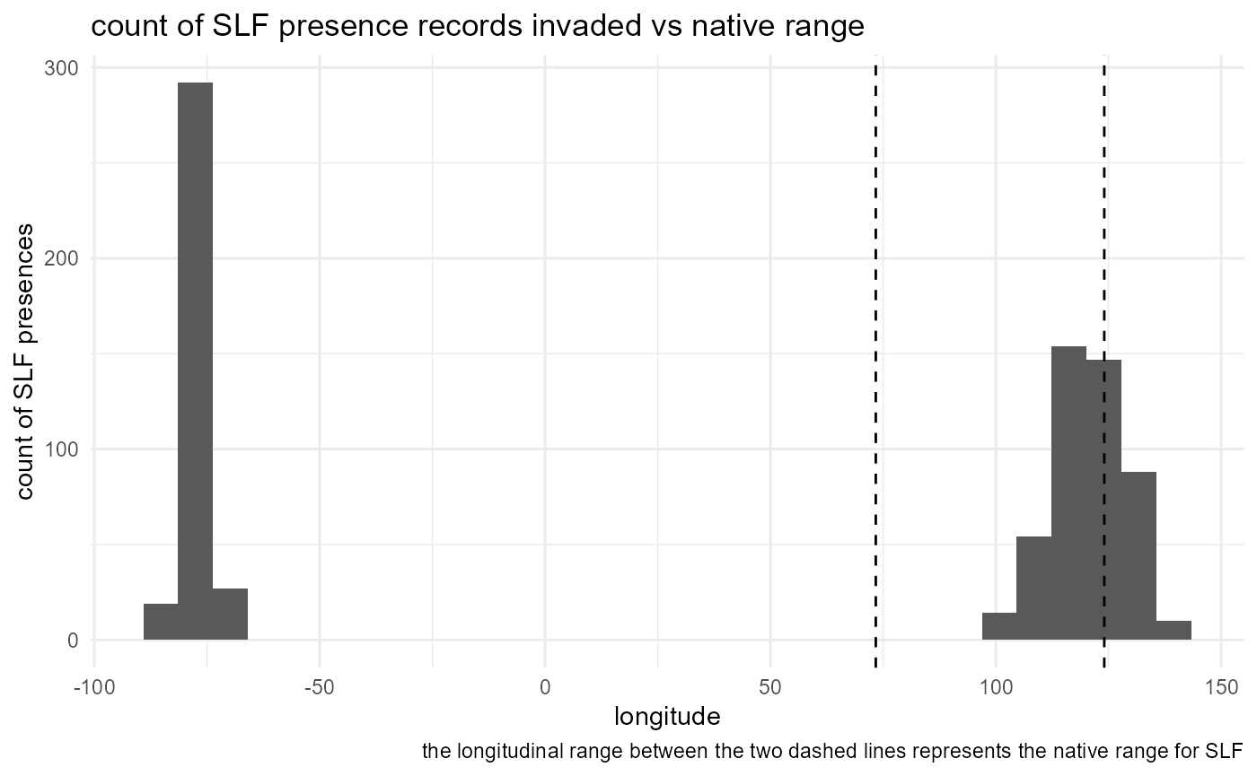
# save output
ggsave(
  SLF_by_longitude, filename = file.path(here::here(), "vignette-outputs", "figures", "SLF_all_coords_final_by_longitude.jpg"),
  height = 8,
  width = 10,
  device = jpeg,
  dpi = 500
  )
The native range includes longitudes between 35 and 105. We can see that most of the SLF presence data are from the invaded ranges of Japan, South Korea or the United States. This is a weakness in the data available and we have given our best effort to account for it by including presence data for China from the literature.
We now have half of the data we need to perform SDM! In the next vignette, we will download historical and projected climate and human impact data, which are the basis of our methods for predicting suitability for Lycorma delicatula.
References
De Bona, S., Barringer, L., Kurtz, P., Losiewicz, J., Parra, G. R., & Helmus, M. R. (2023). lydemapr: An R package to track the spread of the invasive spotted lanternfly (Lycorma delicatula, White 1845) (Hemiptera, Fulgoridae) in the United States. NeoBiota, 86, 151–168. https://doi.org/10.3897/neobiota.86.101471
GBIF Occurrence Download https://doi.org/10.15468/dl.59gndc Accessed from R via rgbif (https://github.com/ropensci/rgbif) on 2024-08-05
Huron, N. A., Behm, J. E., & Helmus, M. R. (2022). Paninvasion severity assessment of a U.S. grape pest to disrupt the global wine market. Communications Biology, 5(1), 655. https://doi.org/10.1038/s42003-022-03580-w
Lin, Y.-S., & Liao, J.-R. (2024). Multifaceted Investigation into the Absence and Potential Invasion of Spotted Lanternfly (Lycorma delicatula) in Taiwan. Research Square. https://doi.org/10.21203/rs.3.rs-4832573/v1
Mestre-Tomás, J. (2024). GeoThinneR: An R package for simple spatial thinning methods in ecological and spatial analysis. R package version 1.0.0, https://github.com/jmestret/GeoThinneR
epsg.io, powered by MapTiler. Transform coordinates - GPS online converter [Internet]. Available from: https://epsg.io/transform#s_srs=4326&t_srs=54017&x=NaN&y=NaN
Coordinate Converter – Polar Geospatial Center [Internet]. Available from: https://applications.pgc.umn.edu/convert/