Bioclim variable rasters: CHELSA
Samuel M. Owens1
2025-07-01
Source:vignettes/020_retrieve_bioclim_variables.Rmd
020_retrieve_bioclim_variables.RmdOverview
This vignette will walk through the process of downloading and tidying these climate data. We will be downloading the data from CHELSA, which is a high-resolution (30 arc-seconds, ~1km) land surface dataset provided by the Swiss Federal Institute for Forest, Snow and Landscape Research. The specific data we are interested in is the suite of 19 “bioclimatic” variables. These bioclim variables are biologically relevant climate features derived from temperature and precipitation. CHELSA also makes the same variables available as climate change predictions, using a subset of the available CMIP6 models. I will use 3 ssp scenarios (126, 370, 585) from the GFDL-ESM4 model (read ahead for an explanation of these).
First, I will download the data from CHELSA into a local library. I will then tidy, harmonize and put the datasets in the proper format for MaxEnt. We will then choose the covariates for our models via an assessment of the level of co-linearity between the rasters. I will also consider biological relevance in selecting the final set of covariates.
Setup
library(tidyverse)  #data manipulation
library(here) #making directory pathways easier on different instances
library(devtools)

# spatial
library(terra)
library(ENMTools) # env covariates colinearity

library(patchwork)
Note: I will be setting the global options of this
document so that only certain code chunks are rendered in the final
.html file. I will set the eval = FALSE so that none of the
code is re-run (preventing files from being overwritten during knitting)
and will simply overwrite this in chunks with plots.
ONLY RUN WITH FINAL RUN THROUGH
1. Retrieve CHELSA bioclim rasters
First, I will download the bioclim data into a local directory. I
recommend downloading these data into a separate directory from this
package. Since I am using a directory outside of the immediate package,
I will create an object to define the file path at the beginning of each
chunk. This pathing will still use here::here() to start at
the package root folder. First, I will download the historical climate
data from CHELSA. The URLs to the bioclim data that were downloaded from
CHELSA are stored in data-raw/CHELSA within the package
directory. I will be using two different versions of the CHELSA bioclim
variables for my analysis:
- Historical- time period 1981-2010
- Climate change predictions- time period 2041-2070, GFDL-ESM4 model, Ssp scenarios 126, 370, and 585.
The CHELSA download directory for each group of bioclim variables also contains 27 other distinct climatologies, available for both historical datasets and climate change models. The URLs for these were also downloaded, as some of them might be applicable to this analysis. For now, we will download the 19 bioclim variables. If you would like to download any of the additional climatologies available from CHELSA, see code for this in the Appendix section of this vignette. Those chunks should be run after the initial run of all chunks before section 2.2. After running these chunks, continue from chunk “loop to tidy rasters” in section 2.2.
1.1 Historical
The best approach I found to download these data was to create a loop to open each URL in a web browser (be ready, as it literally just opens whatever URLs are selected from the list in a browser).
if(FALSE) {

  # historical data
  chelsa_historic_URLs <- read_table(file = file.path(here::here(), "data-raw", "CHELSA", "chelsa_1981-2010_bioclim_URLs.txt"),
                                col_names = FALSE) %>%
    as.data.frame() %>%
    dplyr::select("X1") %>%
    dplyr::rename("URL" = "X1")

  # select only URLs I am interested in
  chelsa_historic_URLs <- slice(.data = chelsa_historic_URLs, 2:20)

  # loop to download historical URLs- I tried utils::download.files, but it would not work with these data
  for(i in 1:nrow(chelsa_historic_URLs)) {

    file.tmp <- chelsa_historic_URLs[i, ]

    utils::browseURL(url = file.tmp)

  }

}
With the current loop construction, these files can only be
downloaded to my PC’s downloads folder, so they will need to be manually
moved to the destination directory (outside of the package root folder
because they are large). These files were stored manually in
maxent/historical_climate_rasters/chelsa2.1_30arcsec/originals.
1.2 CMIP6
Next, I will download data from the provided CMIP6 models. I will be downloading data for different SSP scenarios (see link for an explanation of these scenarios). These ssp scenarios represent different assumptions about global development and greenhouse gas emissions. I will be using the ssp scenarios 126, 370, and 585. 126 represents a more ideal scenario where all countries are cooperating to reduce emissions. 370 represents a middle-high emissions scenario, coupled with an emphasis on regional rivalry and global conflict (which reduce cooperation and drive up emissions). 585 represents a high greenhouse gas emissions scenario where countries are cooperating and improving infrastructure, but there is no emphasis on reducing emissions.
I will use the GFDL-ESM4
CMIP6 model from NOAA. According to the CHELSA documentation, if all
five available models are not used together, then CMIP6 model usage
should follow the given priority (see documentation linked above). These
climate rasters should be moved to their respective folders within
maxent/future_climate_rasters/chelsa2.1_30arcsec once the
download is complete.
SSP126
if(FALSE) {

  # ssp370 data
  chelsa_126_URLs <- read_table(
    file = file.path(here::here(), "data-raw", "CHELSA", "chelsa_2041-2070_GFDL-ESM4_ssp126_bioclim_URLs.txt"),
    col_names = FALSE
    ) %>%
    as.data.frame() %>%
    dplyr::select("X1") %>%
    dplyr::rename("URL" = "X1")


  # select only URLs I am interested in
  chelsa_126_URLs <- slice(.data = chelsa_126_URLs, 1:19)

  # loop to download ssp126 URLs
  for(i in 1:nrow(chelsa_126_URLs)) {

    file.tmp <- chelsa_126_URLs[i, ]

    utils::browseURL(url = file.tmp)

  }

}
SSP370
if(FALSE) {

  # ssp370 data
  chelsa_370_URLs <- read_table(file = file.path(here::here(), "data-raw", "CHELSA", "chelsa_2041-2070_GFDL-ESM4_ssp370_bioclim_URLs.txt"),
                                col_names = FALSE) %>%
    as.data.frame() %>%
    dplyr::select("X1") %>%
    dplyr::rename("URL" = "X1")


  # select only URLs I am interested in
  chelsa_370_URLs <- slice(.data = chelsa_370_URLs, 1:19)

  # loop to download ssp370 URLs
  for(i in 1:nrow(chelsa_370_URLs)) {

    file.tmp <- chelsa_370_URLs[i, ]

    utils::browseURL(url = file.tmp)

  }

}
SSP585
if(FALSE) {

  # ssp370 data
  chelsa_585_URLs <- read_table(
    file = file.path(here::here(), "data-raw", "CHELSA", "chelsa_2041-2070_GFDL-ESM4_ssp585_bioclim_URLs.txt"),
    col_names = FALSE
    ) %>%
    as.data.frame() %>%
    dplyr::select("X1") %>%
    dplyr::rename("URL" = "X1")


  # select only URLs I am interested in
  chelsa_585_URLs <- slice(.data = chelsa_585_URLs, 1:19)

  # loop to download ssp370 URLs
  for(i in 1:nrow(chelsa_585_URLs)) {

    file.tmp <- chelsa_585_URLs[i, ]

    utils::browseURL(url = file.tmp)

  }

}
2. Tidy for MaxEnt
Next, I need to tidy these rasters for MaxEnt. I will need to mask
any data that is over the oceans or other bodies of water. I will also
need to create downsized versions of these variables that can be used in
step 3 to assess the level of correlation between the different
variables. Lastly, I will rename the files and convert them to the
required .ascii format for MaxEnt.
I will mask the CHELSA bioclim rasters using the worldclim version of
bio1, annual mean temperature (mask). The worldclim version
has the continents already cut out, making it a good choice for the
masking. I will use the chelsa bio1 version (main) as a
reference to resample the new layers after setting the CRS and
extent.
2.1 Load in files
First, I will load in the reference layers
# set path to external directory
mypath <- file.path(here::here() %>%
                          dirname(),
                        "maxent/historical_climate_rasters")
# 1st chelsa bioclim layer as reference
ref_chelsa_bio1_main <- terra::rast(x = file.path(mypath, "chelsa2.1_30arcsec", "originals", "CHELSA_bio1_1981-2010_V.2.1.tif"))
ref_wc_bio1_mask <- terra::rast(x = file.path(mypath, "wc2.1_30arcsec", "originals", "wc2.1_30s_bio_1.tif"))We will get a list of the files that I need to modify. We will also create an object containing the new names assigned to the files to simplify the naming.
# set path to external directory
mypath <- file.path(here::here() %>%
                          dirname(),
                        "maxent/historical_climate_rasters/chelsa2.1_30arcsec")
# I will load in the files and then get the new names I would like to give them

# load in bioclim layers to be cropped- the original .tif files
env.files <- list.files(path = file.path(mypath, "originals"), pattern = "\\.tif$", full.names = TRUE)


# output file names
output.files <- list.files(path = file.path(mypath, "originals"), pattern = "\\.tif$", full.names = FALSE) %>%
  # get rid of filetype endings
  gsub(pattern = ".tif", replacement = "") %>%
  # crop off ending
  gsub(pattern = "_V.2.1", replacement = "") %>%
  tolower()
# more edits to file names
output.files <- output.files %>%
  gsub(pattern = "chelsa_", replacement = "")
Note In this version of the vignette, I have isolated only the variables I selected for the final analysis. If you would like to tidy and compare all variables, simply skip this next chunk.
if(TRUE) {

  env.files <- grep("bio2|bio11|bio12|bio15", env.files, value = TRUE)

  output.files <- grep("bio2|bio11|bio12|bio15", output.files, value = TRUE)

}
Now that we have our files and reference layers loaded in and names chosen, we can begin reformatting these layers.
2.2 Prepare reference layers
In this chunk, we will create 2 reference layers.
ref_chelsa_bio1_main will be used for resampling the data,
while ref_wc_bio1_mask will be used for masking. First, I
will crop the layers, set their origins, and resample them to the same
resolution. I will also keep the rasters consistently to
EPSG:4326 for now.
# resolutions
res(ref_chelsa_bio1_main)
res(ref_wc_bio1_mask)
# they are identical

# ext of the reference layers
ext(ref_chelsa_bio1_main)
ext(ref_wc_bio1_mask)
# the extents will need to be corrected

terra::crs(ref_chelsa_bio1_main, parse = TRUE)
terra::crs(ref_wc_bio1_mask, parse = TRUE)
# crs of reference layers is epsg:4326 so no change needed

# check origin
terra::origin(ref_chelsa_bio1_main)
terra::origin(ref_wc_bio1_mask)
# the origin of ref_wc_bio1_mask will need to be changed to match the others
I will need to change the origin and extent of these reference
layers. I will crop them to the same extent first, then unify their
origins. Their extents will be matched to the smallest,
ref_wc_bio1_mask, while their origins will be matched to
the bioclim layer ref_chelsa_bio1_main.
# set extent
# set ext to the smallest whole number shared between the layers
ext.obj <- terra::ext(-179, 179, -89, 83.9)
#  main layer for future cropping, crop to new ext
ref_chelsa_bio1_main <- terra::crop(x = ref_chelsa_bio1_main, y = ext.obj)
#  a mask layer specifically for the cropping and masking
ref_wc_bio1_mask <- terra::crop(x = ref_wc_bio1_mask, y = ext.obj)

# unify origins
# set origin of ref_wc_bio1_mask
terra::origin(ref_wc_bio1_mask) <- c(-0.0001396088, -0.0001392488)
# resample mask to origin of main layer- most rasters will already have the origin of the bio1 layer
ref_wc_bio1_mask <- terra::resample(x = ref_wc_bio1_mask, y = ref_chelsa_bio1_main, method = "bilinear", threads = TRUE)

# check
terra::ext(ref_chelsa_bio1_main)
terra::ext(ref_wc_bio1_mask)
terra::origin(ref_chelsa_bio1_main)
terra::origin(ref_wc_bio1_mask)
Before any visualization (in later vignettes), these layers will be
projected to an equal-area projection. I have chosen the Behrmann cylindrical equal-area
projection, ESRI:54017. Our analysis emphasizes
distributional areas, so use of an equal-area projection is important
for preserving and calculating area correctly.
crs("EPSG:4326", parse = TRUE)## [1] "GEOGCRS[\"WGS 84\","
## [2] " ENSEMBLE[\"World Geodetic System 1984 ensemble\","
## [3] " MEMBER[\"World Geodetic System 1984 (Transit)\"],"
## [4] " MEMBER[\"World Geodetic System 1984 (G730)\"],"
## [5] " MEMBER[\"World Geodetic System 1984 (G873)\"],"
## [6] " MEMBER[\"World Geodetic System 1984 (G1150)\"],"
## [7] " MEMBER[\"World Geodetic System 1984 (G1674)\"],"
## [8] " MEMBER[\"World Geodetic System 1984 (G1762)\"],"
## [9] " MEMBER[\"World Geodetic System 1984 (G2139)\"],"
## [10] " MEMBER[\"World Geodetic System 1984 (G2296)\"],"
## [11] " ELLIPSOID[\"WGS 84\",6378137,298.257223563,"
## [12] " LENGTHUNIT[\"metre\",1]],"
## [13] " ENSEMBLEACCURACY[2.0]],"
## [14] " PRIMEM[\"Greenwich\",0,"
## [15] " ANGLEUNIT[\"degree\",0.0174532925199433]],"
## [16] " CS[ellipsoidal,2],"
## [17] " AXIS[\"geodetic latitude (Lat)\",north,"
## [18] " ORDER[1],"
## [19] " ANGLEUNIT[\"degree\",0.0174532925199433]],"
## [20] " AXIS[\"geodetic longitude (Lon)\",east,"
## [21] " ORDER[2],"
## [22] " ANGLEUNIT[\"degree\",0.0174532925199433]],"
## [23] " USAGE["
## [24] " SCOPE[\"Horizontal component of 3D system.\"],"
## [25] " AREA[\"World.\"],"
## [26] " BBOX[-90,-180,90,180]],"
## [27] " ID[\"EPSG\",4326]]"
crs("ESRI:54017", parse = TRUE)## [1] "PROJCRS[\"World_Behrmann\","
## [2] " BASEGEOGCRS[\"WGS 84\","
## [3] " DATUM[\"World Geodetic System 1984\","
## [4] " ELLIPSOID[\"WGS 84\",6378137,298.257223563,"
## [5] " LENGTHUNIT[\"metre\",1]]],"
## [6] " PRIMEM[\"Greenwich\",0,"
## [7] " ANGLEUNIT[\"Degree\",0.0174532925199433]]],"
## [8] " CONVERSION[\"World_Behrmann\","
## [9] " METHOD[\"Lambert Cylindrical Equal Area\","
## [10] " ID[\"EPSG\",9835]],"
## [11] " PARAMETER[\"Latitude of 1st standard parallel\",30,"
## [12] " ANGLEUNIT[\"Degree\",0.0174532925199433],"
## [13] " ID[\"EPSG\",8823]],"
## [14] " PARAMETER[\"Longitude of natural origin\",0,"
## [15] " ANGLEUNIT[\"Degree\",0.0174532925199433],"
## [16] " ID[\"EPSG\",8802]],"
## [17] " PARAMETER[\"False easting\",0,"
## [18] " LENGTHUNIT[\"metre\",1],"
## [19] " ID[\"EPSG\",8806]],"
## [20] " PARAMETER[\"False northing\",0,"
## [21] " LENGTHUNIT[\"metre\",1],"
## [22] " ID[\"EPSG\",8807]]],"
## [23] " CS[Cartesian,2],"
## [24] " AXIS[\"(E)\",east,"
## [25] " ORDER[1],"
## [26] " LENGTHUNIT[\"metre\",1]],"
## [27] " AXIS[\"(N)\",north,"
## [28] " ORDER[2],"
## [29] " LENGTHUNIT[\"metre\",1]],"
## [30] " USAGE["
## [31] " SCOPE[\"Not known.\"],"
## [32] " AREA[\"World.\"],"
## [33] " BBOX[-90,-180,90,180]],"
## [34] " ID[\"ESRI\",54017]]"
esri_54017_origin <- terra::project(x = ref_chelsa_bio1_main, y = "ESRI:54017", method = "bilinear", threads = TRUE)

# check new UTM units
terra::origin(esri_54017_origin)
terra::res(esri_54017_origin)
terra::ext(esri_54017_origin)

# need to redefine ext.obj for new crs
ext.obj_transformed <- terra::ext(-17271057.5661649, 17271138.5730376, -7340730.14787058, 7300285.39497913)
The origin of the reference layers in the new crs is
332.2808, 349.4412 (measured in UTMs). The resolution of
the new reference layer is 787.4796, 787.4796. The extent
of the new projection is
-17271057.5661649, 17271138.5730376, -7340730.14787058, 7300285.39497913
Finally, I will reproject the main reference layer to the new CRS,
ESRI:54017. The mask layer will stay in
EPSG:4326 because it is used before the reprojection
step.
#reproject as a reference layer used later
ref_chelsa_bio1_main_4326 <- ref_chelsa_bio1_main

# main
ref_chelsa_bio1_main <- terra::project(x = ref_chelsa_bio1_main, y = "ESRI:54017", method = "bilinear", threads = TRUE)
2.3 Tidying historical data
Here is where we get into tidying the data. We will crop the rasters
using the extent object created from the reference layers. We will
follow up the cropping with masking, which will convert cells in
x that do not have a value in worldclim’s bio 1 variable to
NAs. I will also ensure the crs is correct and resample the
rasters. The rasters will be resampled to the resolution of wordlclim
bio 1 so they have the same resolution. The output files will be saved
in v1.
mypath <- file.path(here::here() %>%
                      dirname(),
                    "maxent/historical_climate_rasters/chelsa2.1_30arcsec")
In this first chunk, I will:
- crop the layers to the correct extent
- mask the layers to the outlines of the continents
- set the CRS to the new equal area projection,
ESRI:54017 - set the origin to match the reference layers
- crop the layers again to ensure the aggregation doesn’t increase the extent
This chunk will take a very long time to run… so maybe find a good book to read.
# view list of filetypes for terra, use .ascii
terra::gdal(drivers = TRUE)

# loop to crop extent for all files
for(a in seq_along(env.files)) {

  # load each raster into temp object
  rast.hold <- terra::rast(env.files[a])


  # begin edits
  # crop new rasters to extent
  rast.hold <- terra::crop(x = rast.hold, y = ext.obj)

  # mask the bioclim layers by worldclim bio 1
  rast.hold <- terra::mask(x = rast.hold, mask = ref_wc_bio1_mask)

  # set origin
  terra::origin(rast.hold) <- c(-0.0001396088, -0.0001392488)

  # project crs to new ESRI:54017
  rast.hold <- terra::project(x = rast.hold, y = "ESRI:54017", method = "bilinear", threads = TRUE)

  # resample to fit the extent/resolution of the main layer global_bio1
  # use bilinear interpolation, since values are continuous
  rast.hold <- terra::resample(x = rast.hold, y = ref_chelsa_bio1_main, method = "bilinear", threads = TRUE)

  # run checks
  terra::res(rast.hold)
  terra::ext(rast.hold)
  terra::origin(rast.hold)
  terra::crs(rast.hold)

  # write out the new resampled rasters!
  terra::writeRaster(
    x = rast.hold,
    filename = file.path(mypath, "v1", paste0(output.files[a], "_global", ".tif")),
    filetype = "GTiff",
    overwrite = FALSE
    )

  # remove object once its done
  rm(rast.hold)

}
test_rast <- terra::rast(x = file.path(mypath, "v1", "bio3_1981-2010_global.tif"))
ext(test_rast)

res(test_rast)
ext(test_rast)
terra::crs(test_rast, parse = TRUE)
terra::origin(test_rast)
We will convert the rasters to the .ascii format
required by MaxEnt.
# directory of files to modify
env.files <- list.files(path = file.path(mypath, "v1"), pattern = "\\.tif$", full.names = TRUE)

# output file names
output.files <- list.files(path = file.path(mypath, "v1"), pattern = "\\.tif$", full.names = FALSE) %>%
  gsub(pattern = ".tif", replacement = ".asc")
Note In this version of the vignette, I have isolated only the variables I selected for the final analysis. If you would like to tidy and compare all variables, simply skip this next chunk.
if(TRUE) {

  env.files <- grep("bio2_1981-2010_global|bio11_1981-2010_global|bio12_1981-2010_global|bio15_1981-2010_global", env.files, value = TRUE)

  output.files <- grep("bio2_1981-2010_global|bio11_1981-2010_global|bio12_1981-2010_global|bio15_1981-2010_global", output.files, value = TRUE)

}
Finally, I will aggregate selected rasters to a lower resolution, with roughly 10km grid cells. We want to aggregate at 10km because we will be downsampling the resolution of our analysis to account for survey bias.
# loop to aggregate and convert to .ascii
for(a in seq_along(env.files)){

  # holding object
  rast.hold <- terra::rast(env.files[a])

  # aggregate to 10km scale. cells are 786.3904m sided squares, so I will aggregate by a factor of 12 so that the rasters will be at about 9.5km (as close as I can get to 10 without going over)
  # the na.rm argument is incredibly important because if any of the cells are NAs, the aggregated cell will be an NA value.
  # take the mean for fun
  rast.hold <- terra::aggregate(x = rast.hold, fact = 12, fun = "mean", na.rm = TRUE, threads = TRUE)

  # crop again to ensure aggregation doesnt increase extent
  # use transformed extent
  rast.hold <- terra::crop(x = rast.hold, y = ext.obj_transformed)

  # write output
  terra::writeRaster(
    x = rast.hold,
    filename = file.path(mypath, "v1_maxent_10km", output.files[a]),
    filetype = "AAIGrid",
    overwrite = FALSE
    )

  # remove object once its done
  rm(rast.hold)

}
These data can now be used in a MaxEnt model!
Create reference layer for geothinning
In the next vignette, I will use a raster to perform geothinning of species distribution data. The package I chose to use CoordinateCleaner requires the use of latitude and longitude data as a georeference. I will create a reference layer for that process by performing the same process above, except that the raster will be projected into the EPSG:4326 projection.
mypath <- file.path(here::here() %>%
                      dirname(),
                    "maxent/historical_climate_rasters/chelsa2.1_30arcsec")
# I will load in the files and then get the new names I would like to give them

# load in bioclim layers to be cropped- the original .tif files
env.files <- list.files(path = file.path(mypath, "originals"), pattern = "\\.tif$", full.names = TRUE)
# only bio 2
env.files <- grep("bio2", env.files, value = TRUE)

# output file names
output.files <- "geothinning_ref_layer_epsg4326_bio2"
This process is exactly the same as above, except that it is
projected into the EPSG:4326 crs.
# view list of filetypes for terra, use .ascii
terra::gdal(drivers = TRUE)

# loop to crop extent for all files
for(a in seq_along(env.files)) {

  # load each raster into temp object
  rast.hold <- terra::rast(env.files[a])


  # begin edits
  # crop new rasters to extent
  rast.hold <- terra::crop(x = rast.hold, y = ext.obj)

  # mask the bioclim layers by worldclim bio 1
  rast.hold <- terra::mask(x = rast.hold, mask = ref_wc_bio1_mask)

  # set origin
  terra::origin(rast.hold) <- c(-0.0001396088, -0.0001392488)

  # project crs to new ESRI:54017
  rast.hold <- terra::project(x = rast.hold, y = "EPSG:4326", method = "bilinear", threads = TRUE)

  # resample to fit the extent/resolution of the main layer global_bio1
  # use bilinear interpolation, since values are continuous
  rast.hold <- terra::resample(x = rast.hold, y = ref_chelsa_bio1_main_4326, method = "bilinear", threads = TRUE)

  # run checks
  terra::res(rast.hold)
  terra::ext(rast.hold)
  terra::origin(rast.hold)
  terra::crs(rast.hold)

  # write out the new resampled rasters!
  terra::writeRaster(
    x = rast.hold,
    filename = file.path(mypath, "v1", paste0(output.files[a], ".tif")),
    filetype = "GTiff",
    overwrite = FALSE
    )

  # remove object once its done
  rm(rast.hold)

}
# get the reference layer
env.files <- list.files(path = file.path(mypath, "v1"), pattern = "geothinning", full.names = TRUE)

# output file name
output.files <- list.files(path = file.path(mypath, "v1"), pattern = "geothinning", full.names = FALSE) %>%
  gsub(pattern = ".tif", replacement = ".asc")
# loop to aggregate and convert to .ascii
for(a in seq_along(env.files)){

  # holding object
  rast.hold <- terra::rast(env.files[a])

  # aggregate to 10km scale. cells are 786.3904m sided squares, so I will aggregate by a factor of 12 so that the rasters will be at about 9.5km (as close as I can get to 10 without going over)
  # the na.rm argument is incredibly important because if any of the cells are NAs, the aggregated cell will be an NA value.
  # take the mean for fun
  rast.hold <- terra::aggregate(x = rast.hold, fact = 12, fun = "mean", na.rm = TRUE, threads = TRUE)

  # crop again to ensure aggregation doesnt increase extent
  # use transformed extent
  rast.hold <- terra::crop(x = rast.hold, y = ext.obj)

  # write output
  terra::writeRaster(
    x = rast.hold,
    filename = file.path(mypath, "v1_maxent_10km", output.files[a]),
    filetype = "AAIGrid",
    overwrite = FALSE
    )

  # remove object once its done
  rm(rast.hold)

}
2.4 Tidying CMIP6 data
Here, we will go through all of the above steps in section 2.3 for the CMIP6 versions of the rasters.
# file path to directory
mypath <- file.path(here::here() %>%
                      dirname(),
                    "maxent/future_climate_rasters/chelsa2.1_30arcsec")
SSP126
First, I will get the file names and create folders to hold the new copies per ssp scenario.
# v1 for tidied rasters
dir.create(file.path(mypath, "2041-2070_ssp126_GFDL", "v1"))

# v1_maxent for the ascii versions
dir.create(file.path(mypath, "2041-2070_ssp126_GFDL", "v1_maxent"))

# 10km aggregated versions of ascii
dir.create(file.path(mypath, "2041-2070_ssp126_GFDL", "v1_maxent_10km"))
# I will load in the files and then get the new names I would like to give them

# load in bioclim layers to be cropped- the original .tif files
env.files <- list.files(path = file.path(mypath, "2041-2070_ssp126_GFDL", "originals"), pattern = "\\.tif$", full.names = TRUE)

# output file names
output.files <- list.files(path = file.path(mypath, "2041-2070_ssp126_GFDL", "originals"), pattern = "\\.tif$", full.names = FALSE) %>%
  # change endings to show these are global raster versions
  gsub(pattern = "_V.2.1.tif", replacement = "") %>%
  # crop out some detail
  gsub(pattern = "-esm4_ssp", replacement = "_") %>%
  tolower()

# more edits to file names
output.files <- output.files %>%
  gsub(pattern = "chelsa_", replacement = "")
Note In this version of the vignette, I have isolated only the variables I selected for the final analysis. If you would like to tidy and compare all variables, simply skip this next chunk.
if(TRUE) {

  env.files <- grep("bio2|bio11|bio12|bio15", env.files, value = TRUE)

  output.files <- grep("bio2|bio11|bio12|bio15", output.files, value = TRUE)

}
tidy
# view list of filetypes for terra, use .ascii
terra::gdal(drivers = TRUE)

# loop to crop extent for all files
for(a in seq_along(env.files)) {

  # load each raster into temp object
  rast.hold <- terra::rast(env.files[a])


  # begin edits
  # crop new rasters to extent
  rast.hold <- terra::crop(x = rast.hold, y = ext.obj)

  # mask the bioclim layer by worldclim bio 1
  rast.hold <- terra::mask(x = rast.hold, mask = ref_wc_bio1_mask)

  # set origin
  terra::origin(rast.hold) <- c(-0.0001396088, -0.0001392488)

  # set crs
  rast.hold <- terra::project(x = rast.hold, y = "ESRI:54017", method = "bilinear", threads = TRUE)

  #resample to fit the extent/resolution of the main layer global_bio1
  #use bilinear interpolation, since values are continuous
  rast.hold <- terra::resample(x = rast.hold, y = ref_chelsa_bio1_main, method = "bilinear", threads = TRUE)


  #write out the new resampled rasters!
  terra::writeRaster(
    x = rast.hold,
    filename = file.path(mypath, "2041-2070_ssp126_GFDL", "v1", paste0(output.files[a], "_global", ".tif")),
    filetype = "GTiff",
    overwrite = FALSE
  )

  # remove object once its done
  rm(rast.hold)

}
test_rast <- terra::rast(x = file.path(mypath, "2041-2070_ssp126_GFDL", "v1", "bio15_2041-2070_gfdl_126_global.tif"))


res(test_rast)
ext(test_rast)
terra::crs(test_rast, parse = TRUE)
terra::origin(test_rast)
# directory of files to modify
env.files <- list.files(path = file.path(mypath, "2041-2070_ssp126_GFDL", "v1"), pattern = "\\.tif$", full.names = TRUE)

# output file names
output.files <- list.files(path = file.path(mypath, "2041-2070_ssp126_GFDL", "v1"), pattern = "\\.tif$", full.names = FALSE) %>%
  gsub(pattern = ".tif", replacement = ".asc")
Note In this version of the vignette, I have isolated only the variables I selected for the final analysis. If you would like to tidy and compare all variables, simply skip this next chunk.
if(TRUE) {

  env.files <- grep("bio2_2041-2070_gfdl_126_global|bio11_2041-2070_gfdl_126_global|bio12_2041-2070_gfdl_126_global|bio15_2041-2070_gfdl_126_global", env.files, value = TRUE)

  output.files <- grep("bio2_2041-2070_gfdl_126_global|bio11_2041-2070_gfdl_126_global|bio12_2041-2070_gfdl_126_global|bio15_2041-2070_gfdl_126_global", output.files, value = TRUE)

}
This code chunk was added later so I will only grab the rasters I need downstream.
# loop to aggregate and convert to .ascii
for(a in seq_along(env.files)){

  # holding object
  rast.hold <- terra::rast(env.files[a])

  # aggregate to 10km scale. cells are 786.3904m sided squares, so I will aggregate by a factor of 12 so that the rasters will be at about 9.5km (as close as I can get to 10 without going over)
  rast.hold <- terra::aggregate(x = rast.hold, fact = 12, fun = "mean", na.rm = TRUE, threads = TRUE)

  # crop again to ensure aggregation doesnt increase extent
  rast.hold <- terra::crop(x = rast.hold, y = ext.obj_transformed)

  # write output
  terra::writeRaster(
    x = rast.hold,
    filename = file.path(mypath, "2041-2070_ssp126_GFDL", "v1_maxent_10km", output.files[a]),
    filetype = "AAIGrid",
    overwrite = FALSE
    )

  # remove object once its done
  rm(rast.hold)

}
3. Assess Colinearity
Now that these different climatologies have been tidied for use, we need to decide which variables are the most logical to use in a model for Lycorma delicatula. This can be done by assessing the level of co-linearity between the variables and assessing their biological relevance to SLF.
Before using any of these climatologies in a MaxEnt model, we need to assess their level of co-linearity (the amount the layers are correlated to each other). I expect that most of them will be, as they are all derived from either temperature or precipitation. I will be using a threshold of 0.7 pearson’s correlation or lower to select which variables I use in downstream models. I will only perform a correlation analysis on the historical versions of the rasters, as the climate change versions of the variables are likely to display the same trends. I will use this analysis to decide what covariates go into both the historical and interpolated (climate change) models.
While it is very important to reduce co-linearity, this cannot be the only metric used to select covariates for species distribution models. The biology of the target species is arguably more important than reducing co-linearity. A MaxEnt model that has not been informed by the biology of Lycorma delicatula will likely produce misleading or wrong predictions of its realized niche. Our process of selecting covariates will also need to be informed by the literature. For example, there is evidence that minimum winter temperature has a significantly negative impact on egg survival (Lee et.al, 2011).
We will downsize the rasters from the v1 folder to
perform a co-linearity analysis between the layers. This will only be
done for the historical variables. We will be using
terra::aggregate() to combine cells in a 2x2 grid fashion
and take the mean of the 4 cells.
mypath <- file.path(here::here() %>%
                      dirname(),
                    "maxent/historical_climate_rasters/chelsa2.1_30arcsec")

#list env layers, load
env.files <- list.files(path = file.path(mypath, "v1"), pattern = "\\.tif$", full.names = TRUE) %>%
  # only grab bioclim variables
  grep(pattern = "bio", value = TRUE)

output.files <- list.files(path = file.path(mypath, "v1"), pattern = "\\.tif$", full.names = FALSE) %>%
  # only grab bioclim variables
  grep(pattern = "bio", value = TRUE)

# loop to downsample rasters for colinearity analysis
# code taken from Huron et.al
for(a in seq_along(env.files)){

  # holding object
  rast.hold <- terra::rast(env.files[a])

  rast.hold <- terra::aggregate(
    rast.hold,
    fact = 2, # downsampling by factor of 2 (read 2 cells deep around cell) and take mean of cells
    fun = "mean", # take mean of these cells
    # expand = TRUE, # a carryover from raster::aggregate, terra does this automatically
    na.rm = TRUE,
    filename = file.path(mypath, "v1_downsampled", output.files[a]),
    overwrite = FALSE
    )

  # remove object once its done
  rm(rast.hold)

}
3.1 create and tidy correlation matrix
We will use ENMTools::raster.cor.matrix() to perform the
correlation analysis. This chunk will also take awhile, so its time to
break out that book again.
if(TRUE){

  mypath <- file.path(here::here() %>%
                        dirname(),
                      "maxent/historical_climate_rasters/chelsa2.1_30arcsec")

  # load downsampled layers and stack for raster.cor.matrix command

  # list of layer paths
  env.files <- list.files(path = file.path(mypath, "v1_downsampled"), pattern = "\\.tif$", full.names = TRUE) %>%
    # only grab bioclim variables
    grep(pattern = "bio", value = TRUE)


  # stack downsampled layers
  env <- c(x = terra::rast(env.files))
  # use nlyr, a command of the function terra::dimensions() to see if stacking was successful
  nlyr(env)


  # create a correlation matrix for picking model layers
  env.cor <- ENMTools::raster.cor.matrix(env = env, method = "pearson")

  # write out correlations as .csv.
  write.csv(
    x = env.cor,
    file = file.path(here::here(), "vignette-outputs", "data-tables", "env_cor_chelsa_downsampled_v3.csv"),
    col.names = TRUE,
    row.names = TRUE
    )

}
The correlation values have been saved as a 19x19 matrix. Now that the values have been saved as a .csv file, we need to tidy the data into a more readable format. We will simplify the column and row names and reorder them. We will also convert the correlations to their absolute values so that we can analyze the differences between the layers on a 0-1 scale.
env.cor2 <- read.csv(file = file.path(here::here(), "vignette-outputs", "data-tables", "env_cor_chelsa_downsampled_v3.csv"))

env.cor2 <- as.data.frame(env.cor2)
# convert rownames column to rownames
row.names(env.cor2) <- env.cor2$X
# get rid of X column
env.cor2 <- env.cor2[, which(names(env.cor2) != "X")]

# reorder columns and take absolute values of correlations
env.cor3 <- env.cor2 %>%
  dplyr::select(order(colnames(.))) %>%
  abs(.)

# simplify colnames
colnames(env.cor3) <- gsub(pattern = "_V.2.1", replacement = "", x = colnames(env.cor3))
colnames(env.cor3) <- gsub(pattern = "_1981.2010", replacement = "", x = colnames(env.cor3))
colnames(env.cor3) <- gsub(pattern = "CHELSA_", replacement = "", x = colnames(env.cor3))
# simplify rownames
rownames(env.cor3) <- gsub(pattern = "_V.2.1", replacement = "", x = rownames(env.cor3))
rownames(env.cor3) <- gsub(pattern = "_1981.2010", replacement = "", x = rownames(env.cor3))
rownames(env.cor3) <- gsub(pattern = "CHELSA_", replacement = "", x = rownames(env.cor3))

# factor levels to order row names
var.names <- c(x = "bio1", "bio2", "bio3", "bio4", "bio5", "bio6", "bio7", "bio8", "bio9", "bio10", "bio11", "bio12", "bio13", "bio14", "bio15", "bio16", "bio17", "bio18", "bio19")

# reorder columns
env.cor4 <- env.cor3 %>%
  dplyr::select(bio1, bio2:bio9, bio10:bio19) %>%
  # reorder rows
  mutate(var = rownames(.)) %>% # add column of row names to reorder
  arrange(factor(var, levels = var.names)) %>%
  dplyr::select(!var) # take out temp column

# write tidied data
write.csv(
  x = env.cor4,
  file = file.path(here::here(), "vignette-outputs", "data-tables", "env_cor_chelsa_downsampled_abs_v3.csv"),
  col.names = TRUE,
  row.names = TRUE
  )
The correlations are now more intuitive to read, so they are ready to be analyzed.
3.2 Covariate selection.
Now that they are in a more readable format and have been converted to an absolute scale, we can create heatmaps to display these values and look for trends. I will create a heatmap of both the raw values and of a threshold of any above 0.7.
env.cor5 <- read.csv(file = file.path(here::here(), "vignette-outputs", "data-tables", "env_cor_chelsa_downsampled_abs_v3.csv"))

row.names(env.cor5) <- env.cor5$X

env.cor5 <- as.matrix(env.cor5[, which(names(env.cor5) != "X")])
# Make into triangle
#env.cor5[upper.tri(env.cor5, diag = FALSE)] <- NA

# pivot correlation heatmap for plotting
# code taken from Huron et.al
env.cor5 <- env.cor5 %>%
  tibble::as_tibble() %>%
  mutate(covar = colnames(.)) %>%
  dplyr::select(covar, everything()) %>% # put covar at front
  pivot_longer(cols = -covar, names_to = "var") %>% # pivot longer for plotting
  dplyr::select(var, covar, everything())
I need to set factor levels for the variable names and how to rename them.
# factor levels to order row names
var.names <- c(x = "bio1", "bio2", "bio3", "bio4", "bio5", "bio6", "bio7", "bio8", "bio9", "bio10", "bio11", "bio12", "bio13", "bio14", "bio15", "bio16", "bio17", "bio18", "bio19")

# factor levels to rename abbreviations to actual names
var.renames <- c(
  "bio1" = "annual mean temperature",
  "bio2" = "mean diurnal range",
  "bio3" = "isothermality",
  "bio4" = "temperature seasonality",
  "bio5"    = "max temp of warmest month",
  "bio6" = "min temp of coldest month",
  "bio7" = "temperature annual range",
  "bio8"    = "mean temp of wettest quarter",
  "bio9" = "mean temp of driest quarter",
  "bio10" = "mean temp of warmest quarter",
  "bio11"   = "mean temp of coldest quarter",
  "bio12" = "annual precipitation",
  "bio13" = "precip of wettest month",
  "bio14" = "precip of driest month",
  "bio15" = "precipitation seasonality",
  "bio16" = "precip of wettest quarter",
  "bio17"   = "precip of driest quarter",
  "bio18" = "precip of warmest quarter",
  "bio19" = "precip of coldest quarter"
)
# plot correlation matrix
(env.cor_plot <- ggplot(data = env.cor5) +
  geom_tile(aes(x = factor(var, levels = var.names), # reorder according to var.names factor obj
                y = factor(covar, levels = var.names),
                fill = value)) +
  viridis::scale_fill_viridis(discrete = FALSE, direction = -1, limits = c(0,1), name = "Correlation", na.value = "white") +
  theme_minimal() +
  guides(x =  guide_axis(angle = 45)) +
  labs(x = "", y = "")  +
  labs(title = "Pearson's correlations: CHELSA bioclim covariate rasters") +
  theme(legend.position = "bottom") +
  scale_y_discrete(labels = var.renames) +
   coord_equal(ratio = 1)
)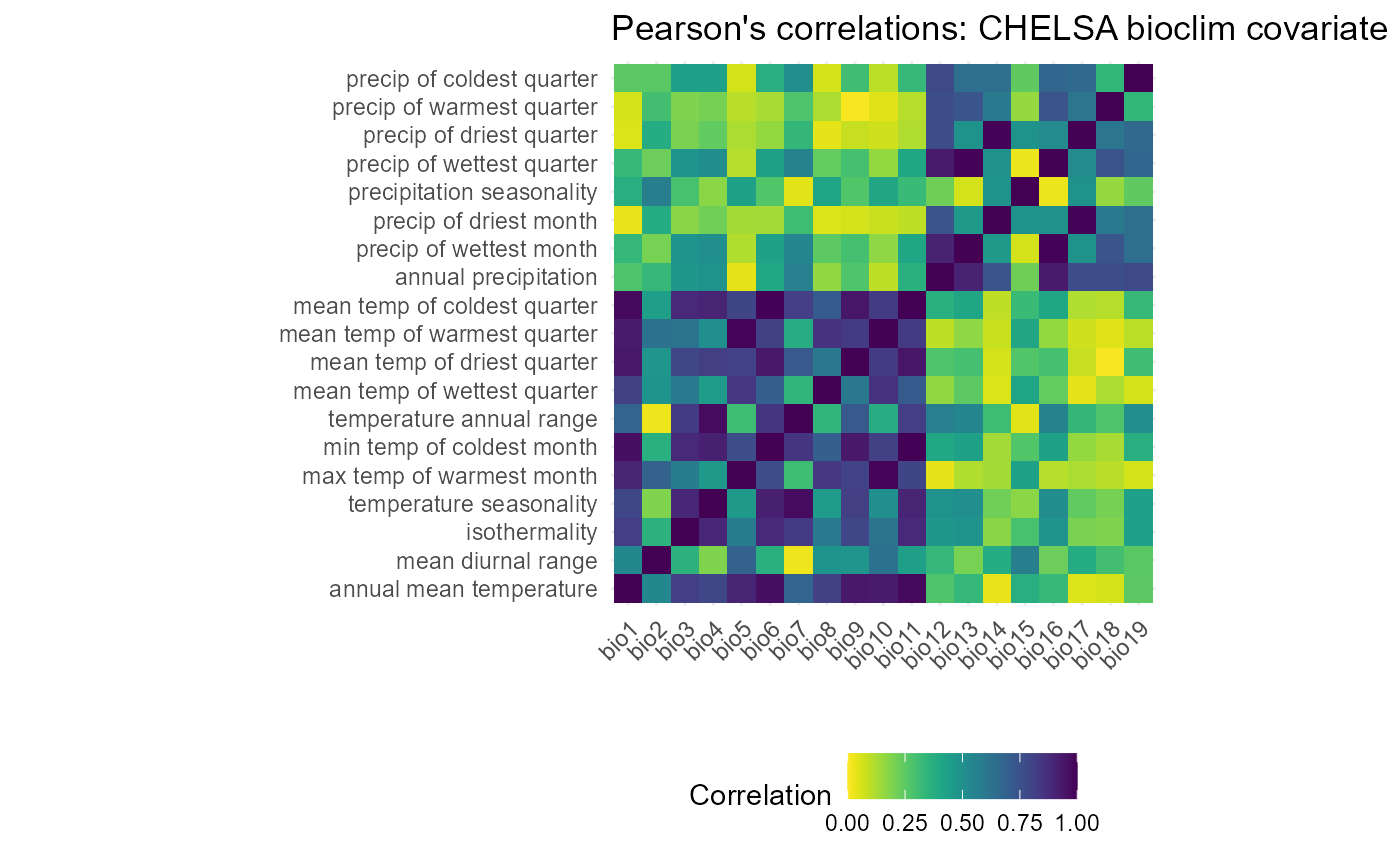
I have found that choosing covariates can be rather ad-hoc, so I developed what I believe is the best-fit methodology for choosing covariates out of much practice. First, I look at the different groupings of covariates (those based on temperature and precipitation) and choose a representative from each group. The ideal representative is highly correlated with most of the others in the group, which indicates its predictive power, and represents a generality of its group (ie, the mean yearly average). In this case, I chose mean temperature of the coldest quarter and precip (bio 11 and 12). Besides its correlation values, mean temp of the coldest quarter is highly impactful for the survival of SLF eggs (Lee et.al, 2011).
I will save this plot and produce a binarized version before I continue choosing variables. This way, the cutoff is clearer and the choice is more obvious.
# save correlation heatmap
ggsave(
  env.cor_plot, filename = file.path(here::here(), "vignette-outputs", "figures", "env_cor_CHELSA_v3.jpg"),
  height = 8,
  width = 10,
  device = jpeg,
  dpi = 500
  )
# binary heatmap

env.cor6 <- env.cor5
# cut values into ranges above and below 0.7
env.cor6$value <- cut(env.cor6$value, breaks = c(0, 0.709, 1), labels = c("0.7 or below", "above 0.7"))

# 0.7 threshold heatmap
(env.cor_binary_plot <- ggplot(data = env.cor6) +
  geom_tile(aes(x = factor(var, levels = var.names), # reorder according to var.names factor obj
                y = factor(covar, levels = var.names),
                fill = value)) +
  theme_minimal() +
  guides(x =  guide_axis(angle = 45),
         fill = guide_legend(title = "Correlation")) +
  labs(x = "", y = "")  +
  labs(
    title = "Pearson's correlations: CHELSA bioclim covariate rasters (binarized)"
    ) +
  scale_fill_manual(values = c("yellow2", "azure4")) +
  theme(legend.position = "bottom") +
  scale_y_discrete(labels = var.renames) +
  coord_equal(ratio = 1)
)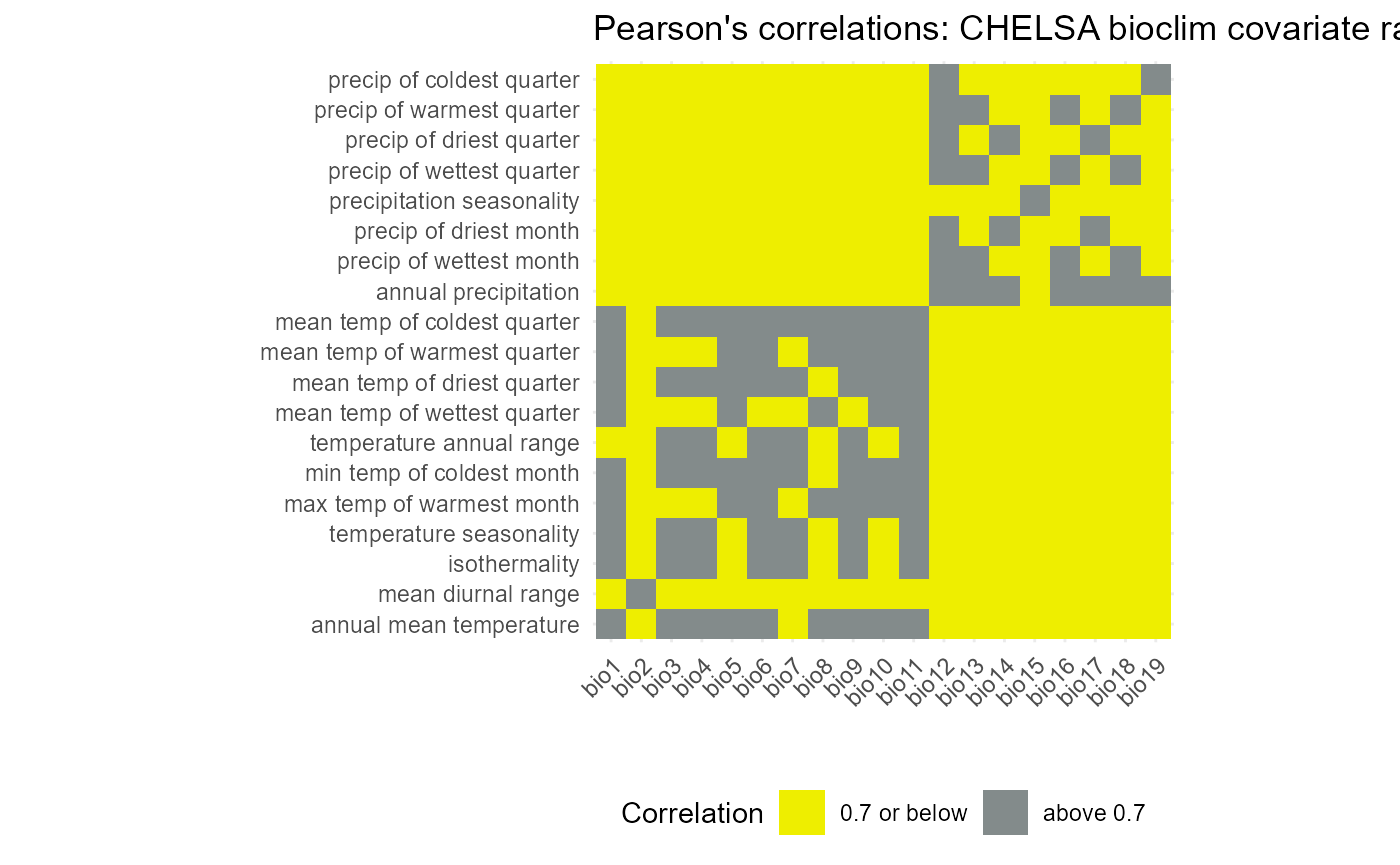
Indeed, the choice is much clearer on this plot. Mean temp of the coldest quarter (bio 11) is above 0.7 correlated with all other temp-based variables, except mean diurnal range (bio 2). Meanwhile, annual precipitation is highly correlated with all precipitation based variables, except precipitation seasonality (bio 12). These two variables were also chosen.
4. Visualize rasters
mypath <- file.path(here::here() %>%
                        dirname(),
                      "maxent/historical_climate_rasters/chelsa2.1_30arcsec")

# load in bio 1
bio1_df <- terra::rast(x = file.path(mypath, "v1_downsampled", "bio1_1981-2010_global.tif")) %>%
  terra::as.data.frame(., xy = TRUE)

bio1_plot <- ggplot() +
  geom_tile(data = bio1_df, aes(x = x, y = y, fill = `CHELSA_bio1_1981-2010_V.2.1`)) +
  xlab("meters easting") +
  ylab("meters northing") +
  theme_minimal() +
  theme(legend.position = "none") +
  labs(title = "CHELSA bio 1") +
  coord_quickmap()

bio1_plot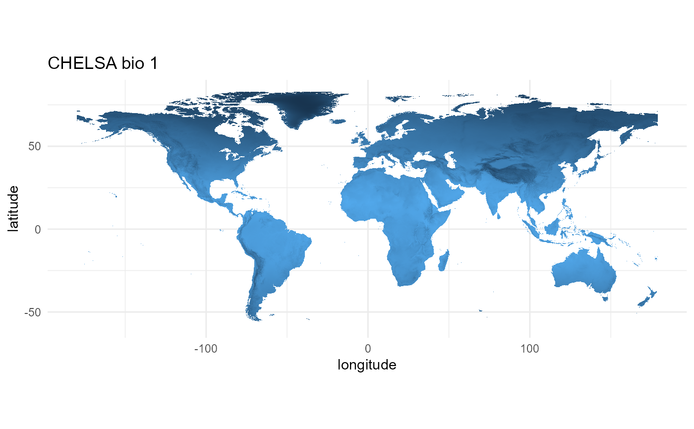
The final 4 variables have been selected for SDM of Lycorma delicatula, which include “mean diurnal range”, “mean temperature of the coldest quarter”, “annual precipitation”, and “precipitation seasonality”. These covariates can be projected for climate change and are biologically relevant to our target species. In the next vignette, we will crop these covariates to the appropriate spatial scale to run a global-scale model. We will also create other necessary datasets for this model.
References
Huron, N. A., Behm, J. E., & Helmus, M. R. (2022). Paninvasion severity assessment of a U.S. grape pest to disrupt the global wine market. Communications Biology, 5(1), 655. https://doi.org/10.1038/s42003-022-03580-w
Karger, D.N., Conrad, O., Böhner, J., Kawohl, T., Kreft, H., Soria-Auza, R.W., Zimmermann, N.E., Linder, P., Kessler, M. (2017). Climatologies at high resolution for the Earth land surface areas. Scientific Data. 4 170122. https://doi.org/10.1038/sdata.2017.122
Karger D.N., Conrad, O., Böhner, J., Kawohl, T., Kreft, H., Soria-Auza, R.W., Zimmermann, N.E, Linder, H.P., Kessler, M. (2018): Data from: Climatologies at high resolution for the earth’s land surface areas. EnviDat. https://doi.org/10.16904/envidat.228.v2.1
Krasting, J. P., John, J. G., Blanton, C., McHugh, C., Nikonov, S., Radhakrishnan, A., Rand, K., Zadeh, N. T., Balaji, V., Durachta, J., Dupuis, C., Menzel, R., Robinson, T., Underwood, S., Vahlenkamp, H., Dunne, K. A., Gauthier, P. P., Ginoux, P., Griffies, S. M., … Zhao, M. (2018). NOAA-GFDL GFDL-ESM4 model output prepared for CMIP6 CMIP [Dataset]. Earth System Grid Federation. https://doi.org/10.22033/ESGF/CMIP6.1407
Lee, J.-S., Kim, I.-K., Koh, S.-H., Cho, S. J., Jang, S.-J., Pyo, S.-H., & Choi, W. I. (2011). Impact of minimum winter temperature on Lycorma delicatula (Hemiptera: Fulgoridae) egg mortality. Journal of Asia-Pacific Entomology, 14(1), 123–125. https://doi.org/10.1016/j.aspen.2010.09.004
Appendix
Additional environmental covariates
Along with the 19 traditional bioclimatic variables, CHELSA has created about 29 additional variables that may help to explain the SLF invasion in N. America. I will include 4 metrics of growing degree day. Several studies have attempted to characterize the lower threshold for egg development and have found numbers between 8-13C (Maino et.al, 2022). Maino et.al also found that egg mortality increased significantly under 10C (Maino et.al, 2022). We will include various measures of degree day with a 10C threshold. Here are the additional variables I will add to the models:
-
GDD10: Growing degree days heat sum above 10°C -
NGD10: Number of growing degree days above 10°C -
GDGFGD10: First growing degree day above 10°C -
GDDLGD10: Last growing degree day above 10°C
Download historical DD variables
if(FALSE) {

  # historical data
  chelsa_historic_URLs <- read_table(file = file.path(here::here(), "data-raw", "CHELSA", "chelsa_1981-2010_bioclim_URLs.txt"),
                                col_names = FALSE) %>%
    as.data.frame() %>%
    dplyr::select("X1") %>%
    dplyr::rename("URL" = "X1")

  # select only DD URLs
  chelsa_historic_URLs <- slice(.data = chelsa_historic_URLs, c(32, 35, 38, 55))

  # loop to download historical URLs
  for(i in 1:nrow(chelsa_historic_URLs)) {

    file.tmp <- chelsa_historic_URLs[i, ]

    utils::browseURL(url = file.tmp)

  }

}
Files were placed in
"maxent/historical_climate_rasters/chelsa2.1_30arcsec/originals".