Create risk maps of each model scale and intersect predictions

Overview

In the last vignette, I applied a weighting factor to the three regional-scale models to create an ensembled mean prediction. I have already created a global-scale model prediction, so now that the regional-scale models have been ensembled, I can directly compare the predictions made by the two modeled scales. Each model in this multi-scale analysis has been projected to the entire globe, so I can now measure the differences between these two models. My goals for application of these models are to look at the predictions for SLF risk of establishment made (A) spatially for globally important winegrowing countries, (B) at the specific locations of globally important viticultural regions, and (C) at the location of known SLF populations. I plan to explore the suitability for SLF via creating a range of outputs:

risk maps
range shift maps
viticultural risk quadrant plots
viticultural risk tables
variable response curves
other summary statistics, including AUC and variable contribution

In this vignette, I will create all mapping outputs to depict the risk of SLF establishment both historically and under future climate scenarios. I will also create a range shift map to show the expansion and contraction of suitable area under climate change. I will create these maps by intersecting the global and regional_ensemble model predictions to create classified (binarized) rasters. The level of agreement between each model prediction will be used to infer the level of SLF establishment risk.

The process will follow this general flow for creating the risk maps:

Create suitable vs unsuitable classes based on the MTSS threshold of both rasters
Convert each model raster to binary (suitable/unsuitable) based on these suitability thresholds
Mosaic the two rasters and sum their values.
Re-classify summed raster as areas where both agree on presence, both agree on absence, or one classifies and the other classifies absent (4 total categories)

I created a consensus MTSS threshold for each model in the previous vignette, which I will use to binarize these rasters. This procedure will be repeated for each ssp scenario and then a mean of the scenarios to produce different predictions based on different climate scenarios. I will also calculate the total area per risk category and raster to show how the change in suitable area might change depending on the ssp scenario.

Finally, I will plot a range shift map to show the expansion and contraction of suitable area per ssp scenario (essentially, the difference between the historical and future predictions).

Setup

# general tools
library(tidyverse)  #data manipulation
library(here) #making directory pathways easier on different instances
# here() starts at the root folder of this package.
library(devtools)
library(common)

# spatial data handling
library(terra) 

# aesthetics
library(viridis)
library(webshot)
library(webshot2)
library(kableExtra)

Note: I will be setting the global options of this document so that only certain code chunks are rendered in the final .html file. I will set the eval = FALSE so that none of the code is re-run (preventing files from being overwritten during knitting) and will simply overwrite this in chunks with plots.

I will load in preset styles for the maps. The regular map_style will be for the continuous suitability maps, while map_style_binarized will be used for specialized binary overlay maps between the regional ensemble and the global models.

map_style <- list(
  xlab("longitude"),
  ylab("latitude"),
  theme_classic(),
  theme(
    # legend
    legend.position = "bottom",
    legend.title = element_text(margin = margin(r = 15, b = 45), hjust = 1),
    legend.text = element_text(margin = margin(t = 10), angle = 35),
    # background
    panel.background = element_rect(fill = "lightblue2",
                                        colour = "lightblue2")
  ),
  scale_x_continuous(expand = c(0, 0)),
  scale_y_continuous(expand = c(0, 0)),
  labs(fill = "Suitability for SLF \n(cloglog)"),
  coord_equal()
)

map_style_binarized <- list(
  xlab("longitude"),
  ylab("latitude"),
  theme_classic(),
  theme(
    # legend
    legend.position = "bottom",
    # background
    panel.background = element_rect(fill = "lightblue2",
                                        colour = "lightblue2")
  ),
  scale_x_continuous(expand = c(0, 0)),
  scale_y_continuous(expand = c(0, 0)),
  coord_equal()
)

mypath <- file.path(here::here() %>% 
                       dirname(),
                     "maxent/models")

Import datasets

I will import the predicted suitability rasters and MTSS thresholds from each of the models. I will stack these rasters and harmonize their naming.

regional ensemble

# historical 
regional_ensemble_1995 <- terra::rast(
  x = file.path(mypath, "slf_regional_ensemble_v1", "ensemble_regional_weighted_mean_globe_1981-2010.asc")
  )


# CMIP6
# ssp126
regional_ensemble_2055_126 <- terra::rast(
  x = file.path(mypath, "slf_regional_ensemble_v1", "ensemble_regional_weighted_mean_globe_2041-2070_GFDL_ssp126.asc")
  )
# ssp370
regional_ensemble_2055_370 <- terra::rast(
  x = file.path(mypath, "slf_regional_ensemble_v1", "ensemble_regional_weighted_mean_globe_2041-2070_GFDL_ssp370.asc")
  )
# ssp585
regional_ensemble_2055_585 <- terra::rast(
  x = file.path(mypath, "slf_regional_ensemble_v1", "ensemble_regional_weighted_mean_globe_2041-2070_GFDL_ssp585.asc")
  )

# the mean of the ssp scenarios
regional_ensemble_2055_ssp_mean <- terra::rast(
  x = file.path(mypath, "slf_regional_ensemble_v1", "ensemble_regional_weighted_mean_globe_2041-2070_GFDL_ssp_averaged.asc")
  )

regional_ensemble_thresholds <- read_csv(file = file.path(mypath, "slf_regional_ensemble_v1", "ensemble_threshold_values.csv"))

# change names
names(regional_ensemble_1995) <- "ensemble_suitability"
# CMIP6
names(regional_ensemble_2055_126) <- "ensemble_suitability"
names(regional_ensemble_2055_370) <- "ensemble_suitability"
names(regional_ensemble_2055_585) <- "ensemble_suitability"
names(regional_ensemble_2055_ssp_mean) <- "ensemble_suitability"

# also convert to df
regional_ensemble_1995_df <- terra::as.data.frame(regional_ensemble_1995, xy = TRUE)
# CMIP6
regional_ensemble_2055_126_df <- terra::as.data.frame(regional_ensemble_2055_126, xy = TRUE)
regional_ensemble_2055_370_df <- terra::as.data.frame(regional_ensemble_2055_370, xy = TRUE)
regional_ensemble_2055_585_df <- terra::as.data.frame(regional_ensemble_2055_585, xy = TRUE)
regional_ensemble_2055_ssp_mean_df <- terra::as.data.frame(regional_ensemble_2055_ssp_mean, xy = TRUE)

Global model

# historical 
global_1995 <- terra::rast(
  x = file.path(mypath, "slf_global_v3", "global_pred_suit_clamped_cloglog_globe_1981-2010_mean.asc")
  )

# CMIP6
# ssp126
global_2055_126 <- terra::rast(
  x = file.path(mypath, "slf_global_v3", "global_pred_suit_clamped_cloglog_globe_2041-2070_GFDL_ssp126_mean.asc")
  )
# ssp370
global_2055_370 <- terra::rast(
  x = file.path(mypath, "slf_global_v3", "global_pred_suit_clamped_cloglog_globe_2041-2070_GFDL_ssp370_mean.asc")
  )
# ssp126
global_2055_585 <- terra::rast(
  x = file.path(mypath, "slf_global_v3", "global_pred_suit_clamped_cloglog_globe_2041-2070_GFDL_ssp585_mean.asc")
  )

# also import mean raster
global_2055_ssp_mean <- terra::rast(
  x = file.path(mypath, "slf_global_v3", "global_pred_suit_clamped_cloglog_globe_2041-2070_GFDL_ssp_averaged.asc")
  )

summary_global <- read_csv(file.path(mypath, "slf_global_v3", "global_summary_all_iterations.csv")) %>%
  dplyr::select(., statistic, mean)

# change names
# historical
names(global_1995) <- "global_suitability"
# CMIP6
names(global_2055_126) <- "global_suitability"
names(global_2055_370) <- "global_suitability"
names(global_2055_585) <- "global_suitability"
names(global_2055_ssp_mean) <- "global_suitability"

# also convert to df
global_1995_df <- terra::as.data.frame(global_1995, xy = TRUE)
# CMIP6
global_2055_126_df <- terra::as.data.frame(global_2055_126, xy = TRUE)
global_2055_370_df <- terra::as.data.frame(global_2055_370, xy = TRUE)
global_2055_585_df <- terra::as.data.frame(global_2055_585, xy = TRUE)
global_2055_ssp_mean_df <- terra::as.data.frame(global_2055_ssp_mean, xy = TRUE)

1. Map cloglog suitability

Before I binarize these mapped predictions, I will plot raw suitability maps from each of the models.

1.1 Mapping helper function

I will try to reduce the amount of repeated code by using a mapping helper function containing the body of the plotting code. This part will remain relatively unchanged each time.

map_cloglog_output <- function(raster.df, raster.value.name, thresh.MTP, thresh.MTSS) {
  
  # raster.df = the dataframe of the raster
  # raster.value.name = the name of the raster values
  # thresh.MTP = the df cell coordinates of the MTP thresh
  # thresh.MTSS = the df cell coordinates of the MTSS thresh
  
  ggplot() +
    # default style object
    map_style +
    # plot raster
    geom_raster(data = raster.df, aes(x = x, y = y, fill = raster.value.name)) +
    # aesthetics
    scale_fill_gradientn(
      # the values of the color divisions: 0, MTP, slightly above MTP, MTSS, slightly above MTSS, 0.5, 0.75, 1
      values = c(
        0, # minimum
        as.numeric(thresh.MTP), # MTP thresh
        as.numeric(thresh.MTP) + 0.0000001, # some small amount more than the MTP
        as.numeric(thresh.MTSS), # MTSS thresh
        as.numeric(thresh.MTSS) + 0.0000001,
        # the rest
        0.5,
        0.75,
        1
        ),
      # these colors taken from viridis color scale D
      # the colors for the divisions in the order: 0, MTP, slightly above MTP, MTSS, slightly above MTSS, 0.5, 0.75, 1
      colors = c("azure4", "azure4", "azure2", "azure2", "#481567FF", "#2D708EFF", "#3CBB75FF", "#FDE725FF"),
      # the tick marks
      breaks = c(0, as.numeric(thresh.MTP), as.numeric(thresh.MTSS), 0.5, 0.75, 1.00),
      # labels for the tick marks
      labels = c("unsuitable", "", paste0(round(as.numeric(thresh.MTSS), 2), "\n(MTSS thresh)"), 0.5, 0.75, 1),
      limits = c(0, 1.0),
      guide = guide_colorbar(frame.colour = "black", ticks.colour = "black", barwidth = 20, draw.ulim = TRUE, draw.llim = TRUE)
      ) 
  
}

1.2 Map cloglog output of models- historical

First, I will map the ensemble of the three regional-scale cloglog outputs.

regional_ensemble_1995_plot <- map_cloglog_output(
  raster.df = regional_ensemble_1995_df, # the dataframe of the raster
  raster.value.name = regional_ensemble_1995_df$ensemble_suitability, # the name of the raster values
  thresh.MTP = regional_ensemble_thresholds[1, 4], # the df cell coordinates of the MTP thresh
  thresh.MTSS = regional_ensemble_thresholds[6, 4] # the df cell coordinates of the MTSS thresh
) +
  # labs
  labs(
    title = "Suitability for SLF in regional model ensemble",
    subtitle = "1981-2010",
    caption = "MTP & MTSS thresholds | clamped"
    ) 

regional_ensemble_1995_plot

## Warning: Raster pixels are placed at uneven horizontal intervals and will be shifted
## ℹ Consider using `geom_tile()` instead.

ggsave(
  regional_ensemble_1995_plot,
  filename = file.path(mypath, "slf_regional_ensemble_v1", "plots", "regional_ensemble_pred_suit_globe_1981-2010.jpg"),
  height = 8,
  width = 12,
  device = jpeg,
  dpi = "retina"
  )

## Warning: Raster pixels are placed at uneven horizontal intervals and will be shifted
## ℹ Consider using `geom_tile()` instead.

I will repeat the same process to map the predictions for each ssp scenario for 2041-2070. I will also mean these scenarios for a final prediction under climate change.

1.3 Map cloglog output of models- CMIP6

ssp mean

Finally, I will plot the mean of the three ssp scenarios. First, the regional ensemble.

## Warning: Raster pixels are placed at uneven horizontal intervals and will be shifted
## ℹ Consider using `geom_tile()` instead.

Now I will plot the global-scale model.

## Warning: Raster pixels are placed at uneven horizontal intervals and will be shifted
## ℹ Consider using `geom_tile()` instead.

2. Create binary threshold maps to infer range filling

Now that I have an idea of what the suitability maps look like before conversion, I will reclassify and combine these maps. I will create matrix objects that will be used to reclassify the output rasters to a binary predictor of suitability. I will use the MTSS (““Maximum Test Sensitivity Plus Specificity”) threshold for each model as the threshold for suitability, with anything below this threshold being considered unsuitable for SLF establishment.

To reclassify, package terra takes a 3-column matrix for its classify() function, which re-classifies groups of values to a single value. I will reclassify anything below the MTSS threshold as one value, and anything above as another.

summary_global

## # A tibble: 52 × 2
##    statistic                        mean
##    <chr>                           <dbl>
##  1 X.Training.samples            578.   
##  2 Regularized.training.gain       3.34 
##  3 Unregularized.training.gain     3.78 
##  4 Iterations                   1818    
##  5 Training.AUC                    0.986
##  6 X.Background.points         20000    
##  7 bio11.contribution             58.8  
##  8 bio12.contribution             19.3  
##  9 bio15.contribution             15.6  
## 10 bio2.contribution               6.34 
## # ℹ 42 more rows

# MTSS value is 0.041

regional_ensemble_thresholds

## # A tibble: 10 × 4
##    thresh time_period CMIP6_model         value
##    <chr>  <chr>       <chr>               <dbl>
##  1 MTP    1981-2010   NA                 0.0128
##  2 MTP    2041-2070   ssp126_GFDL        0.0128
##  3 MTP    2041-2070   ssp370_GFDL        0.0128
##  4 MTP    2041-2070   ssp585_GFDL        0.0128
##  5 MTP    2041-2070   ssp_mean_GFDL-ESM4 0.0128
##  6 MTSS   1981-2010   NA                 0.241 
##  7 MTSS   2041-2070   ssp126_GFDL        0.241 
##  8 MTSS   2041-2070   ssp370_GFDL        0.241 
##  9 MTSS   2041-2070   ssp585_GFDL        0.241 
## 10 MTSS   2041-2070   ssp_mean_GFDL-ESM4 0.241

# MTSS value is ~0.241

I will create separate classification matrices for each of the global and regional-scale ensemble outputs. The reason for having two separate matrices is because I will need to differentiate between a “suitable” spot on the global and regional rasters. Base-2 binary offers an intuitive system for creating these class differences. I will encode the rasters into base-2 binary so that the end result is 4 categories of values (the idea for this was found in this forum).

I will encode the cloglog output of MaxEnt into these values:

Model and suitability	cloglog range	binary value	output value
Regional unsuitable	0 - 0.241	00000001	1
Regional suitable	0.2411 - 1	00000010	2
Global unsuitable	0 - 0.041	00000100	4
Global suitable	0.0411 - 1	00001000	8

By encoding the rasters into base-2, I have created only 4 possible values of the raster layers, which can be translated into 4 categories:

Unsuitable Agreement = 5 (00000101)
Suitable Agreement = 10 (00001010)
unsuitable regional/suitable global = 9 (00001001)
Suitable regional/unsuitable global = 6 (00000110)

I will also interpret these categories in terms of risk of SLF suitability. These categories can be thought of as:

Unsuitable Agreement = low risk Suitable Agreement = high risk Suitable regional/unsuitable global = adaptive risk unsuitable regional/suitable global = imminent risk

Gallien et al, 2012 interprets these categories in terms of specific ecological mechanisms, but we prefer to interpret them in terms of the risk for SLF.

2.1 convert output rasters to binary predictors

I will walk through this workflow initially, but will functionalize it after this to avoid repeating it four more times.

historical

To convert the rasters to binary predictors of presence / absence, first I will create the classification matrices needed by the classify() function. Before converting, lets check the range of values.

# get the range of the values in the raster
terra::minmax(global_1995) %>%
  format(., scientific = FALSE) # convert scientific notation to decimals

##     global_suitability  
## min "0.0000000001702356"
## max "1.0000000000000000"

# get the range of the values in the raster
terra::minmax(regional_ensemble_1995) %>%
  format(., scientific = FALSE)

##     ensemble_suitability
## min "0.0000001336334"   
## max "0.7144208550453"

# all looks good

Now I will create the classification rasters. I will pull these from their respective .csv files.

# create regional suitability value matrix for terra
regional_ensemble_classes <- data.frame(
  from = c(0, as.numeric(regional_ensemble_thresholds[6, 4]) + 0.0000000001), # add a small amount to the lower end of the 2nd range
  to = c(as.numeric(regional_ensemble_thresholds[6, 4]), 1), 
  becomes = c(strtoi(00000001, base = 2), strtoi(00000010, base = 2)) # the strtoi function converts to base-2, becomes 1 and 2
)

global_classes <- data.frame(
  from = c(0, as.numeric(summary_global[42, 2]) + 0.0000000001),
  to = c(as.numeric(summary_global[42, 2]), 1), 
  becomes = c(strtoi(00000100, base = 2), strtoi(00001000, base = 2)) # becomes 4 and 8
)

Now I can reclassify the MaxEnt outputs. I will load in the averaged predictions for the global and regional models for the time period 1981-2010. I will reclassify their values based on the two matrices above. This chunk might take some time to run.

# regional
# reclassify and write regional raster
regional_ensemble_1995_classified <- terra::classify(
  x = regional_ensemble_1995, 
  rcl = regional_ensemble_classes,
  right = NA, # close both ends of the range of classification values
  others = strtoi(00000001, base = 2), # make it the unsuitable value if not in this range
  filename = file.path(mypath, "working_dir", "slf_regional_ensemble_v1_binarized_1981-2010.asc"), # also write to file
  filetype = "AAIGrid",
  overwrite = FALSE
  ) 

# global
# reclassify and write global raster
global_1995_classified <- terra::classify(
  x = global_1995, 
  rcl = global_classes, 
  right = NA, 
  others = strtoi(00000100, base = 2), 
  filename = file.path(mypath, "working_dir", "slf_global_v3_binarized_1981-2010.asc"), 
  filetype = "AAIGrid",
  overwrite = FALSE
  )

I will run a few error checks to ensure that the binarization process worked.

# take minmax
terra::minmax(global_1995_classified) %>%
  format(., scientific = FALSE)

terra::minmax(regional_ensemble_1995_classified) %>%
  format(., scientific = FALSE)

# all good

# check unique values
unique(values(global_1995_classified))
unique(values(regional_ensemble_1995_classified))

Now that the rasters have been converted to binary, we will visualize them to ensure that the process worked. Since the same process was done to both the regional and global models, I will only plot the regional model.

# load in binary raster just created and convert to df
regional_ensemble_1995_classified_df <- terra::rast(
  x = file.path(mypath, "working_dir", "slf_regional_ensemble_v1_binarized_1981-2010.asc")
  ) %>%
  terra::as.data.frame(., xy = TRUE) #%>%
  #na.omit()

# now, create vectors of values used to manually edit the scale of the plot
# the possible values of the scale and their order
breaks.obj <- unique(regional_ensemble_1995_classified_df$ensemble_suitability)
# labels for the values
labels.obj <- c("regional unsuitable", "regional suitable")
# vector of colors to classify scale
values.obj <- c(
  "azure4",
  "darkblue"
)

# plot regional binary
ggplot() +
  geom_raster(data = regional_ensemble_1995_classified_df, aes(x = x, y = y, fill = as.factor(ensemble_suitability))) +
  labs(title = "Binarized suitability for 'regional_ensemble' model") +
  scale_discrete_manual(
    name = "suitability for SLF",
    values = values.obj,
    breaks = breaks.obj,
    labels = labels.obj,
    aesthetics = "fill",
    ) +
  map_style_binarized

## Warning: Raster pixels are placed at uneven horizontal intervals and will be shifted
## ℹ Consider using `geom_tile()` instead.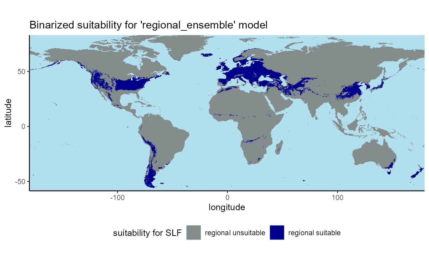

I will perform the same operation as above for the predicted climate change rasters from 2041-2070 (ssp126, 370, 585 and the mean of these).

The helper function below, classify_matrix(), will create the object needed to classify each raster into the binary-based classes I outlined above.

helper function- terra classify

classify_matrix <- function(thresh, model.scale) {
  
  # thresh = the threshold for suitability in that model
  # model = either of "global" or "regional"
  
  # the strtoi function converts a number to base-2
  
  # regional model classes
  if (model.scale == "regional") {
    
    data.frame(
      from = c(0, as.numeric(thresh) + 0.0000000001), # add a small amount to the lower end of the 2nd range
      to = c(as.numeric(thresh), 1), 
      becomes = c(strtoi(00000001, base = 2), strtoi(00000010, base = 2)) # becomes 1 and 2
)
    
    # otherwise, go with global model
  } else if (model.scale == "global") {
    
    data.frame(
      from = c(0, as.numeric(thresh) + 0.0000000001),
      to = c(as.numeric(thresh), 1), 
      becomes = c(strtoi(00000100, base = 2), strtoi(00001000, base = 2)) # becomes 4 and 8
    )
    
  }
  
  }

# get the range of the values in the raster
terra::minmax(global_2055_126) %>%
  format(., scientific = FALSE) # convert scientific notation to decimals


# get the range of the values in the raster
terra::minmax(regional_ensemble_2055_126) %>%
  format(., scientific = FALSE)

# global
global_classes <- classify_matrix(
  thresh = summary_global[42, 2],
  model.scale = "global"
)

# regional ensemble
regional_ensemble_classes <- classify_matrix(
  thresh = regional_ensemble_thresholds[7, 4],
  model.scale = "regional"
)

# regional
# reclassify and write regional raster
regional_ensemble_2055_126_classified <- terra::classify(
  x = regional_ensemble_2055_126, 
  rcl = regional_ensemble_classes,
  right = NA, # close both ends of the range of classification values
  others = strtoi(00000001, base = 2), # make it the unsuitable value if not in this range
  filename = file.path(mypath, "working_dir", "slf_regional_ensemble_v1_binarized_2041-2070_ssp126_GFDL.asc"), # also write to file
  filetype = "AAIGrid",
  overwrite = FALSE
  ) 

# global
# reclassify and write global raster
global_2055_126_classified <- terra::classify(
  x = global_2055_126, 
  rcl = global_classes, 
  right = NA, 
  others = strtoi(00000100, base = 2), 
  filename = file.path(mypath, "working_dir", "slf_global_v3_binarized_2041-2070_ssp126_GFDL.asc"), 
  filetype = "AAIGrid",
  overwrite = FALSE
  )

# take minmax
terra::minmax(global_2055_126_classified) %>%
  format(., scientific = FALSE)

terra::minmax(regional_ensemble_2055_126_classified) %>%
  format(., scientific = FALSE)

# all good

# check unique values
unique(values(global_2055_126_classified))
unique(values(regional_ensemble_2055_126_classified))

# load in binary raster just created and convert to df
regional_ensemble_2055_126_classified_df <- terra::rast(
  x = file.path(mypath, "working_dir", "slf_regional_ensemble_v1_binarized_2041-2070_ssp126_GFDL.asc")
  ) %>%
  terra::as.data.frame(., xy = TRUE)

# now, create vectors of values used to manually edit the scale of the plot
# the possible values of the scale and their order
breaks.obj <- unique(regional_ensemble_2055_126_classified_df$ensemble_suitability)
# labels for the values
labels.obj <- c("regional unsuitable", "regional suitable")
# vector of colors to classify scale
values.obj <- c(
  "azure4",
  "darkblue"
)

# plot regional binary
ggplot() +
  geom_raster(data = regional_ensemble_2055_126_classified_df, aes(x = x, y = y, fill = as.factor(ensemble_suitability))) +
  labs(
    title = "Binarized suitability for 'regional_ensemble' model",
    subtitle = "projected to 2041-2070 | ssp126 | GFDL"
    ) +
  scale_discrete_manual(
    name = "suitability for SLF",
    values = values.obj,
    breaks = breaks.obj,
    labels = labels.obj,
    aesthetics = "fill"
    ) +
  map_style_binarized

# get the range of the values in the raster
terra::minmax(global_2055_370) %>%
  format(., scientific = FALSE) # convert scientific notation to decimals


# get the range of the values in the raster
terra::minmax(regional_ensemble_2055_370) %>%
  format(., scientific = FALSE)

# global
global_classes <- classify_matrix(
  thresh = summary_global[42, 2],
  model.scale = "global"
)

# regional ensemble
regional_ensemble_classes <- classify_matrix(
  thresh = regional_ensemble_thresholds[8, 4],
  model.scale = "regional"
)

# regional
# reclassify and write regional raster
regional_ensemble_2055_370_classified <- terra::classify(
  x = regional_ensemble_2055_370, 
  rcl = regional_ensemble_classes,
  right = NA, # close both ends of the range of classification values
  others = strtoi(00000001, base = 2), # make it the unsuitable value if not in this range
  filename = file.path(mypath, "working_dir", "slf_regional_ensemble_v1_binarized_2041-2070_ssp370_GFDL.asc"), # also write to file
  filetype = "AAIGrid",
  overwrite = FALSE
  ) 

# global
# reclassify and write global raster
global_2055_370_classified <- terra::classify(
  x = global_2055_370, 
  rcl = global_classes, 
  right = NA, 
  others = strtoi(00000100, base = 2), 
  filename = file.path(mypath, "working_dir", "slf_global_v3_binarized_2041-2070_ssp370_GFDL.asc"), 
  filetype = "AAIGrid",
  overwrite = FALSE
  )

# take minmax
terra::minmax(global_2055_370_classified) %>%
  format(., scientific = FALSE)

terra::minmax(regional_ensemble_2055_370_classified) %>%
  format(., scientific = FALSE)

# all good

# check unique values
unique(values(global_2055_370_classified))
unique(values(regional_ensemble_2055_370_classified))

# load in binary raster just created and convert to df
regional_ensemble_2055_370_classified_df <- terra::rast(
  x = file.path(mypath, "working_dir", "slf_regional_ensemble_v1_binarized_2041-2070_ssp370_GFDL.asc")
  ) %>%
  terra::as.data.frame(., xy = TRUE)

# now, create vectors of values used to manually edit the scale of the plot
# the possible values of the scale and their order
breaks.obj <- unique(regional_ensemble_2055_370_classified_df$ensemble_suitability)
# labels for the values
labels.obj <- c("regional unsuitable", "regional suitable")
# vector of colors to classify scale
values.obj <- c(
  "azure4",
  "darkblue"
)

# plot regional binary
ggplot() +
  geom_raster(data = regional_ensemble_2055_370_classified_df, aes(x = x, y = y, fill = as.factor(ensemble_suitability))) +
  labs(
    title = "Binarized suitability for 'regional_ensemble' model",
    subtitle = "projected to 2041-2070 | ssp370 | GFDL"
    ) +
  scale_discrete_manual(
    name = "suitability for SLF",
    values = values.obj,
    breaks = breaks.obj,
    labels = labels.obj,
    aesthetics = "fill"
    ) +
  map_style_binarized

# get the range of the values in the raster
terra::minmax(global_2055_585) %>%
  format(., scientific = FALSE) # convert scientific notation to decimals


# get the range of the values in the raster
terra::minmax(regional_ensemble_2055_585) %>%
  format(., scientific = FALSE)

# global
global_classes <- classify_matrix(
  thresh = summary_global[42, 2],
  model.scale = "global"
)

# regional ensemble
regional_ensemble_classes <- classify_matrix(
  thresh = regional_ensemble_thresholds[9, 4],
  model.scale = "regional"
)

# regional
# reclassify and write regional raster
regional_ensemble_2055_585_classified <- terra::classify(
  x = regional_ensemble_2055_585, 
  rcl = regional_ensemble_classes,
  right = NA, # close both ends of the range of classification values
  others = strtoi(00000001, base = 2), # make it the unsuitable value if not in this range
  filename = file.path(mypath, "working_dir", "slf_regional_ensemble_v1_binarized_2041-2070_ssp585_GFDL.asc"), # also write to file
  filetype = "AAIGrid",
  overwrite = FALSE
  ) 

# global
# reclassify and write global raster
global_2055_585_classified <- terra::classify(
  x = global_2055_585, 
  rcl = global_classes, 
  right = NA, 
  others = strtoi(00000100, base = 2), 
  filename = file.path(mypath, "working_dir", "slf_global_v3_binarized_2041-2070_ssp585_GFDL.asc"), 
  filetype = "AAIGrid",
  overwrite = FALSE
  )

# take minmax
terra::minmax(global_2055_585_classified) %>%
  format(., scientific = FALSE)

terra::minmax(regional_ensemble_2055_585_classified) %>%
  format(., scientific = FALSE)

# all good

# check unique values
unique(values(global_2055_585_classified))
unique(values(regional_ensemble_2055_585_classified))

# load in binary raster just created and convert to df
regional_ensemble_2055_585_classified_df <- terra::rast(
  x = file.path(mypath, "working_dir", "slf_regional_ensemble_v1_binarized_2041-2070_ssp585_GFDL.asc")
  ) %>%
  terra::as.data.frame(., xy = TRUE)

# now, create vectors of values used to manually edit the scale of the plot
# the possible values of the scale and their order
breaks.obj <- unique(regional_ensemble_2055_585_classified_df$ensemble_suitability)
# labels for the values
labels.obj <- c("regional unsuitable", "regional suitable")
# vector of colors to classify scale
values.obj <- c(
  "azure4",
  "darkblue"
)

# plot regional binary
ggplot() +
  geom_raster(data = regional_ensemble_2055_585_classified_df, aes(x = x, y = y, fill = as.factor(ensemble_suitability))) +
  labs(
    title = "Binarized suitability for 'regional_ensemble' model",
    subtitle = "projected to 2041-2070 | ssp585 | GFDL"
    ) +
  scale_discrete_manual(
    name = "suitability for SLF",
    values = values.obj,
    breaks = breaks.obj,
    labels = labels.obj,
    aesthetics = "fill"
    ) +
  map_style_binarized

ssp mean

# get the range of the values in the raster
terra::minmax(global_2055_ssp_mean) %>%
  format(., scientific = FALSE) # convert scientific notation to decimals

##     global_suitability   
## min "0.00000000003642224"
## max "1.00000000000000000"

# get the range of the values in the raster
terra::minmax(regional_ensemble_2055_ssp_mean) %>%
  format(., scientific = FALSE)

##     ensemble_suitability
## min "0.0000001578022"   
## max "0.7055209279060"

# global
global_classes <- classify_matrix(
  thresh = summary_global[42, 2],
  model.scale = "global"
)

# regional ensemble
regional_ensemble_classes <- classify_matrix(
  thresh = regional_ensemble_thresholds[10, 4],
  model.scale = "regional"
)

# regional
# reclassify and write regional raster
regional_ensemble_2055_ssp_mean_classified <- terra::classify(
  x = regional_ensemble_2055_ssp_mean, 
  rcl = regional_ensemble_classes,
  right = NA, # close both ends of the range of classification values
  others = strtoi(00000001, base = 2), # make it the unsuitable value if not in this range
  filename = file.path(mypath, "working_dir", "slf_regional_ensemble_v1_binarized_2041-2070_ssp_mean_GFDL.asc"), # also write to file
  filetype = "AAIGrid",
  overwrite = FALSE
  ) 

# global
# reclassify and write global raster
global_2055_ssp_mean_classified <- terra::classify(
  x = global_2055_ssp_mean, 
  rcl = global_classes, 
  right = NA, 
  others = strtoi(00000100, base = 2), 
  filename = file.path(mypath, "working_dir", "slf_global_v3_binarized_2041-2070_ssp_mean_GFDL.asc"), 
  filetype = "AAIGrid",
  overwrite = FALSE
  )

# take minmax
terra::minmax(global_2055_ssp_mean_classified) %>%
  format(., scientific = FALSE)

terra::minmax(regional_ensemble_2055_ssp_mean_classified) %>%
  format(., scientific = FALSE)

# all good

# check unique values
unique(values(global_2055_ssp_mean_classified))
unique(values(regional_ensemble_2055_ssp_mean_classified))

Now lets plot the binarized mean of the ssp scenarios.

# load in binary raster just created and convert to df
regional_ensemble_2055_ssp_mean_classified_df <- terra::rast(
  x = file.path(mypath, "working_dir", "slf_regional_ensemble_v1_binarized_2041-2070_ssp_mean_GFDL.asc")
  ) %>%
  terra::as.data.frame(., xy = TRUE)

# now, create vectors of values used to manually edit the scale of the plot
# the possible values of the scale and their order
breaks.obj <- unique(regional_ensemble_2055_ssp_mean_classified_df$ensemble_suitability)
# labels for the values
labels.obj <- c("regional unsuitable", "regional suitable")
# vector of colors to classify scale
values.obj <- c(
  "azure4",
  "darkblue"
)

# plot regional binary
ggplot() +
  geom_raster(data = regional_ensemble_2055_ssp_mean_classified_df, aes(x = x, y = y, fill = as.factor(ensemble_suitability))) +
  labs(
    title = "Binarized suitability for 'regional_ensemble' model",
    subtitle = "projected to 2041-2070 | mean of ssp126, 370, 585 | GFDL"
    ) +
  scale_discrete_manual(
    name = "suitability for SLF",
    values = values.obj,
    breaks = breaks.obj,
    labels = labels.obj,
    aesthetics = "fill"
    ) +
  map_style_binarized

## Warning: Raster pixels are placed at uneven horizontal intervals and will be shifted
## ℹ Consider using `geom_tile()` instead.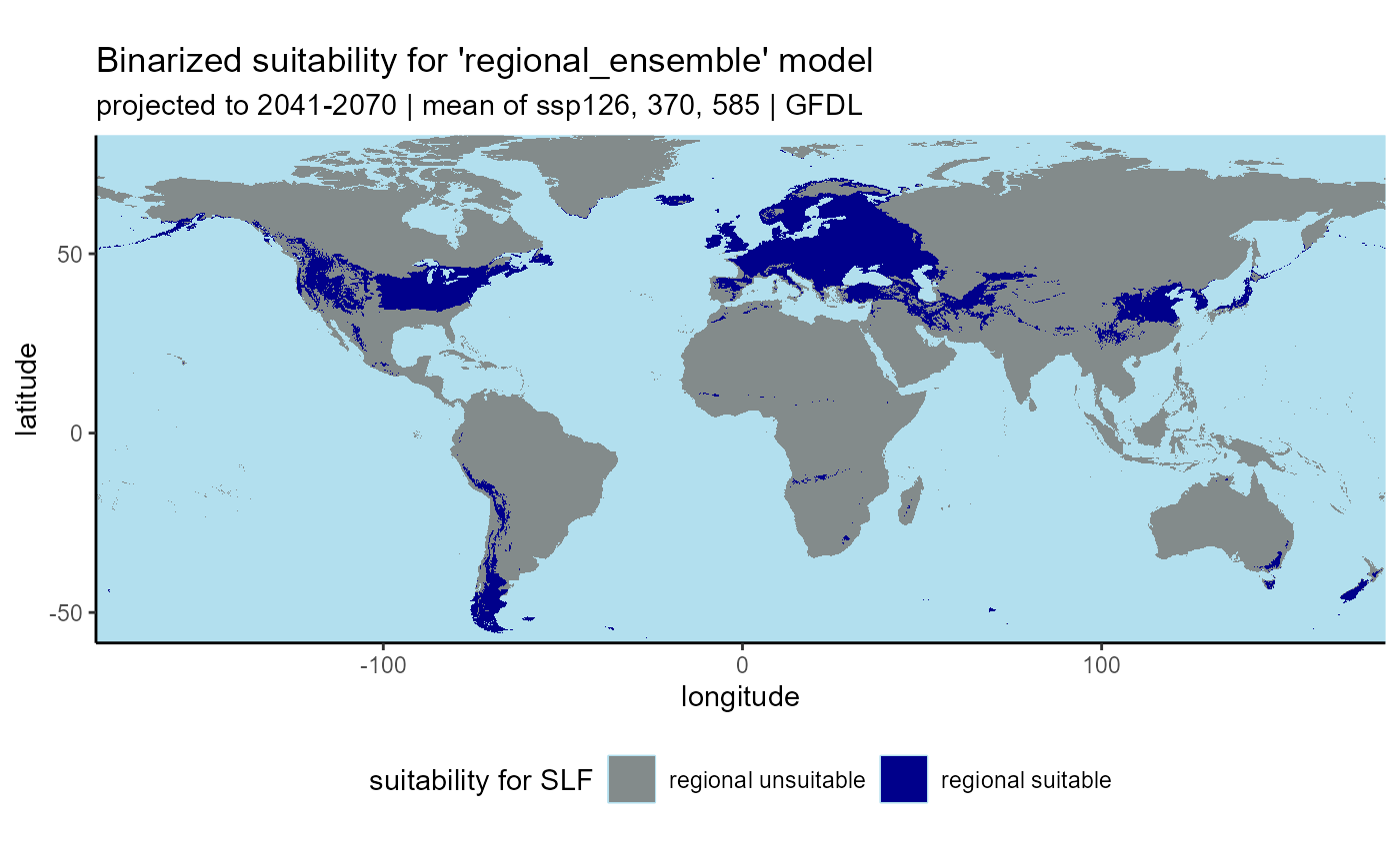

2.2 Mosaic rasters and produce map

From the plots, we see that the binary conversion worked. Next, I will need to stack the reclassified global and regional rasters and add them into a single raster output. This should give me a final raster with 4 classes:

SLF suitability	raster value
Unsuitable Agreement	5
Suitable Agreement	10
unsuitable regional/suitable global	9
Suitable regional/unsuitable global	6

The mosaic function combines spatRasters that overlap in extent into a new raster, via the function specified (addition, in this case). I will run through this workflow for the historical rasters, then will functionalize the plotting for the ssp scenarios.

historical

global_1995_classified <- terra::rast(x = file.path(mypath, "working_dir", "slf_global_v3_binarized_1981-2010.asc"))

regional_ensemble_1995_classified <- terra::rast(x = file.path(mypath, "working_dir", "slf_regional_ensemble_v1_binarized_1981-2010.asc"))

# overlay and combine rasters by summing values
slf_binarized_1995 <- terra::mosaic(
  global_1995_classified, regional_ensemble_1995_classified, # rasters
  fun = "sum", 
  filename = file.path(mypath, "working_dir", "slf_binarized_summed_1981-2010.asc"),
  overwrite = FALSE,
  wopt = list(progress = 1)) # progress bar

I will prepare plotting objects.

slf_binarized_1995 <- terra::rast(x = file.path(mypath, "working_dir", "slf_binarized_summed_1981-2010.asc")) 
# rename values
names(slf_binarized_1995) <- "global_regional_binarized"
# convert to df
slf_binarized_1995_df <- terra::as.data.frame(slf_binarized_1995, xy = TRUE) #%>%
 # na.omit()

# check for the number of unique values in the raster values column
unique(slf_binarized_1995_df$global_regional_binarized)

## [1]  5  6 10  9

# it seems that the reclassification worked! Lets map it to be sure.

# now, create vectors of values used to manually edit the scale of the plot
# the possible values of the scale and their order
breaks.obj <- c(5, 9, 6, 10) # i manually ordered these
# labels for the values
labels.obj <- c("low", "moderate", "high", "extreme")
# vector of colors to classify scale
values.obj <- c("azure4", "gold", "darkorange", "darkred")

slf_binarized_1995_plot <- ggplot() +
  geom_raster(data = slf_binarized_1995_df, aes(x = x, y = y, fill = as.factor(global_regional_binarized))) +
  labs(
    title = "Projected risk of Lycorma delicatula invasion globally",
    subtitle = "1981-2010"
    ) +
  scale_discrete_manual(
    name = "projected risk",
    values = values.obj,
    breaks = breaks.obj,
    labels = labels.obj,
    aesthetics = "fill",
    guide = guide_colorsteps(frame.colour = "black", ticks.colour = "black", barwidth = 20, draw.ulim = TRUE, draw.llim = TRUE)
    ) +
  map_style_binarized +
  guides(fill = guide_legend(nrow = 1, byrow = TRUE)) +
  theme(legend.key = element_rect(color = "black"))

ggsave(
  slf_binarized_1995_plot, 
  filename = file.path(here::here(), "vignette-outputs", "figures", "slf_binarized_summed_1981-2010.jpg"),
  height = 8, 
  width = 12,
  device = jpeg,
  dpi = "retina"
  )

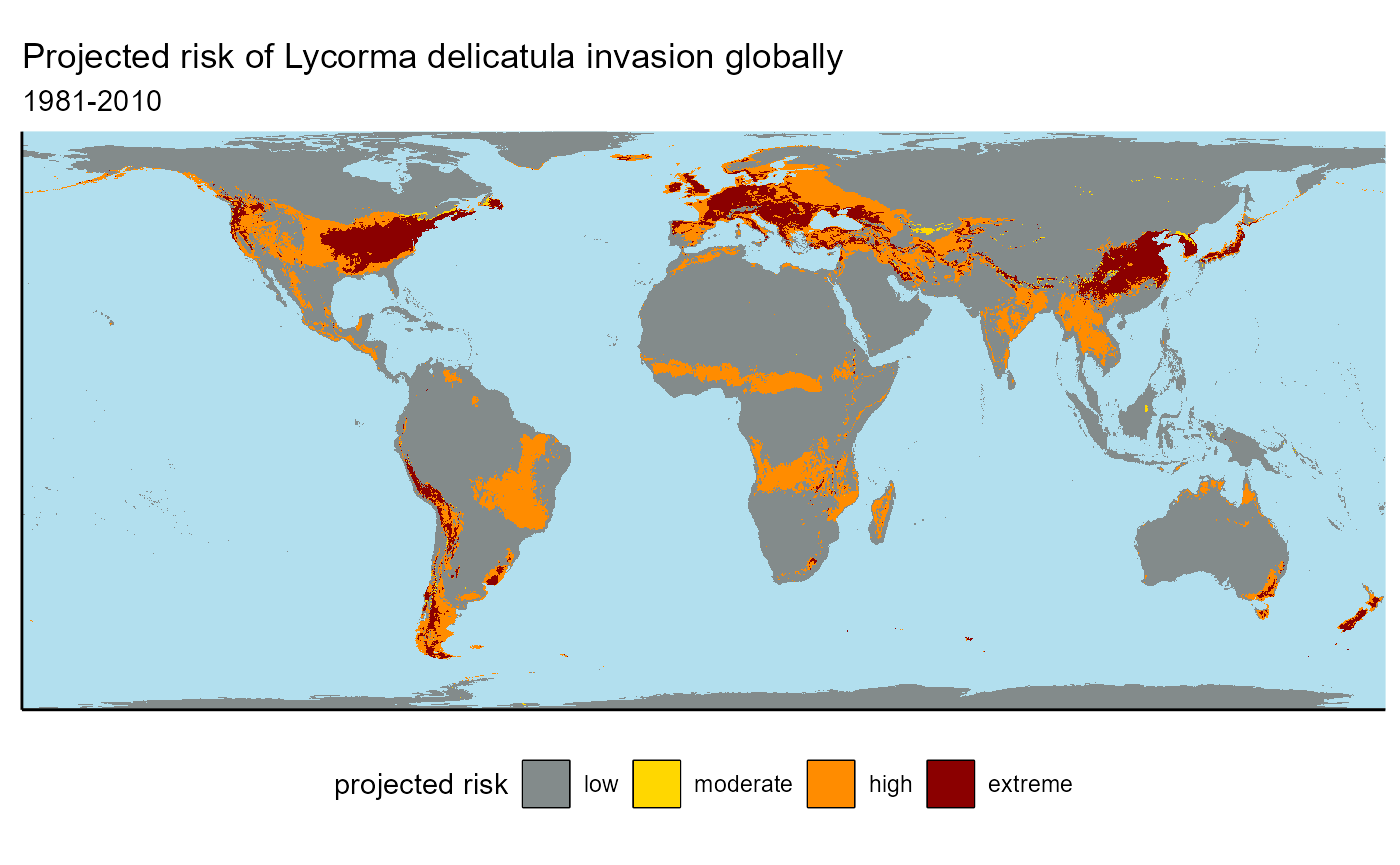
helper function- binary raster plotting

Now that I have run through the process once, I will functionalize the plotting process for the ssp scenarios to save time and lines of code.

# first, create vectors of values used to manually edit the scale of the plot
# the possible values of the scale and their order
breaks.obj <- c(5, 9, 6, 10) # i manually ordered these
# labels for the values
labels.obj <- c("low", "moderate", "high", "extreme")
# vector of colors to classify scale
values.obj <- c("azure4", "gold", "darkorange", "darkred")


# function
plot_binary <- function(raster.df) {
  
  # raster.df = data frame of the raster to be plotted
  
  ggplot() +
    # default map style
    map_style_binarized +
    # raster layer
    geom_raster(data = raster.df, aes(x = x, y = y, fill = as.factor(global_regional_binarized))) +
    # custom discrete scale
    scale_discrete_manual(
      name = "projected risk",
      # use objects outlined above
      values = values.obj,
      breaks = breaks.obj,
      labels = labels.obj,
      aesthetics = "fill",
      guide = guide_colorsteps(frame.colour = "black", ticks.colour = "black", barwidth = 20, draw.ulim = TRUE, draw.llim = TRUE)
      ) +
    # other theme customizations
    guides(fill = guide_legend(nrow = 1, byrow = TRUE)) +
    theme(legend.key = element_rect(color = "black")) 
  
}

global_2055_126_classified <- terra::rast(x = file.path(mypath, "working_dir", "slf_global_v3_binarized_2041-2070_ssp126_GFDL.asc"))

regional_ensemble_2055_126_classified <- terra::rast(x = file.path(mypath, "working_dir", "slf_regional_ensemble_v1_binarized_2041-2070_ssp126_GFDL.asc"))

# overlay and combine rasters by summing values
slf_binarized_2055_126 <- terra::mosaic(
  global_2055_126_classified, regional_ensemble_2055_126_classified, # rasters
  fun = "sum", 
  filename = file.path(mypath, "working_dir", "slf_binarized_summed_2041-2070_ssp126_GFDL.asc"),
  overwrite = FALSE,
  wopt = list(
    progress = 1, # progress bar
    names = "global_regional_binarized" # layer name, change in function if this changes
    )  
  )

slf_binarized_2055_126 <- terra::rast(x = file.path(mypath, "working_dir", "slf_binarized_summed_2041-2070_ssp126_GFDL.asc")) 

# convert to df
slf_binarized_2055_126_df <- terra::as.data.frame(slf_binarized_2055_126, xy = TRUE) #%>%
 # na.omit()

# check for the number of unique values in the raster values column
unique(slf_binarized_2055_126_df$global_regional_binarized)
# it seems that the reclassification worked! Lets map it to be sure.

slf_binarized_2055_126_plot <- plot_binary(
  raster.df = slf_binarized_2055_126_df
) +
  # labels
  labs(
    title = "Projected risk of Lycorma delicatula invasion globally under climate change",
    subtitle = "2041-2070 | ssp126 GFDL-ESM4"
    )

ggsave(
  slf_binarized_2055_126_plot, 
  filename = file.path(here::here(), "vignette-outputs", "figures", "slf_binarized_summed_2041-2070_ssp126_GFDL.jpg"),
  height = 8, 
  width = 12,
  device = jpeg,
  dpi = "retina"
  )

global_2055_370_classified <- terra::rast(x = file.path(mypath, "working_dir", "slf_global_v3_binarized_2041-2070_ssp370_GFDL.asc"))

regional_ensemble_2055_370_classified <- terra::rast(x = file.path(mypath, "working_dir", "slf_regional_ensemble_v1_binarized_2041-2070_ssp370_GFDL.asc"))

# overlay and combine rasters by summing values
slf_binarized_2055_370 <- terra::mosaic(
  global_2055_370_classified, regional_ensemble_2055_370_classified, # rasters
  fun = "sum", 
  filename = file.path(mypath, "working_dir", "slf_binarized_summed_2041-2070_ssp370_GFDL.asc"),
  overwrite = FALSE,
  wopt = list(
    progress = 1, # progress bar
    names = "global_regional_binarized" # layer name, change in function if this changes
    )  
  )

slf_binarized_2055_370 <- terra::rast(x = file.path(mypath, "working_dir", "slf_binarized_summed_2041-2070_ssp370_GFDL.asc")) 

# convert to df
slf_binarized_2055_370_df <- terra::as.data.frame(slf_binarized_2055_370, xy = TRUE) #%>%
 # na.omit()

# check for the number of unique values in the raster values column
unique(slf_binarized_2055_370_df$global_regional_binarized)
# it seems that the reclassification worked! Lets map it to be sure.

slf_binarized_2055_370_plot <- plot_binary(
  raster.df = slf_binarized_2055_370_df
) +
  # labels
  labs(
    title = "Projected risk of Lycorma delicatula invasion globally under climate change",
    subtitle = "2041-2070 | ssp370 GFDL-ESM4"
    )

ggsave(
  slf_binarized_2055_370_plot, 
  filename = file.path(here::here(), "vignette-outputs", "figures", "slf_binarized_summed_2041-2070_ssp370_GFDL.jpg"),
  height = 8, 
  width = 12,
  device = jpeg,
  dpi = "retina"
  )

global_2055_585_classified <- terra::rast(x = file.path(mypath, "working_dir", "slf_global_v3_binarized_2041-2070_ssp585_GFDL.asc"))

regional_ensemble_2055_585_classified <- terra::rast(x = file.path(mypath, "working_dir", "slf_regional_ensemble_v1_binarized_2041-2070_ssp585_GFDL.asc"))

# overlay and combine rasters by summing values
slf_binarized_2055_585 <- terra::mosaic(
  global_2055_585_classified, regional_ensemble_2055_585_classified, # rasters
  fun = "sum", 
  filename = file.path(mypath, "working_dir", "slf_binarized_summed_2041-2070_ssp585_GFDL.asc"),
  overwrite = FALSE,
  wopt = list(
    progress = 1, # progress bar
    names = "global_regional_binarized" # layer name, change in function if this changes
    )  
  )

slf_binarized_2055_585 <- terra::rast(x = file.path(mypath, "working_dir", "slf_binarized_summed_2041-2070_ssp585_GFDL.asc")) 

# convert to df
slf_binarized_2055_585_df <- terra::as.data.frame(slf_binarized_2055_585, xy = TRUE) #%>%
 # na.omit()

# check for the number of unique values in the raster values column
unique(slf_binarized_2055_585_df$global_regional_binarized)
# it seems that the reclassification worked! Lets map it to be sure.

slf_binarized_2055_585_plot <- plot_binary(
  raster.df = slf_binarized_2055_585_df
) +
  # labels
  labs(
    title = "Projected risk of Lycorma delicatula invasion globally under climate change",
    subtitle = "2041-2070 | ssp585 GFDL-ESM4"
    )

ggsave(
  slf_binarized_2055_585_plot, 
  filename = file.path(here::here(), "vignette-outputs", "figures", "slf_binarized_summed_2041-2070_ssp585_GFDL.jpg"),
  height = 8, 
  width = 12,
  device = jpeg,
  dpi = "retina"
  )

ssp mean

global_2055_ssp_mean_classified <- terra::rast(x = file.path(mypath, "working_dir", "slf_global_v3_binarized_2041-2070_ssp_mean_GFDL.asc"))

regional_ensemble_2055_ssp_mean_classified <- terra::rast(x = file.path(mypath, "working_dir", "slf_regional_ensemble_v1_binarized_2041-2070_ssp_mean_GFDL.asc"))

# overlay and combine rasters by summing values
slf_binarized_2055_ssp_mean <- terra::mosaic(
  global_2055_ssp_mean_classified, regional_ensemble_2055_ssp_mean_classified, # rasters
  fun = "sum", 
  filename = file.path(mypath, "working_dir", "slf_binarized_summed_2041-2070_ssp_mean_GFDL.asc"),
  overwrite = FALSE,
  wopt = list(
    progress = 1, # progress bar
    names = "global_regional_binarized" # layer name, change in function if this changes
    )  
  )

slf_binarized_2055_ssp_mean <- terra::rast(x = file.path(mypath, "working_dir", "slf_binarized_summed_2041-2070_ssp_mean_GFDL.asc")) 

# convert to df
slf_binarized_2055_ssp_mean_df <- terra::as.data.frame(slf_binarized_2055_ssp_mean, xy = TRUE) #%>%
 # na.omit()

# check for the number of unique values in the raster values column
unique(slf_binarized_2055_ssp_mean_df$global_regional_binarized)

## [1]  5  6 10  9

# it seems that the reclassification worked! Lets map it to be sure.

slf_binarized_2055_ssp_mean_plot <- plot_binary(
  raster.df = slf_binarized_2055_ssp_mean_df
) +
  # labels
  labs(
    title = "Projected risk of Lycorma delicatula invasion globally under climate change",
    subtitle = "2041-2070 | mean of ssp126, ssp370 and ssp585, GFDL-ESM4"
    )

ggsave(
  slf_binarized_2055_ssp_mean_plot, 
  filename = file.path(here::here(), "vignette-outputs", "figures", "slf_binarized_summed_2041-2070_ssp_mean_GFDL.jpg"),
  height = 8, 
  width = 12,
  device = jpeg,
  dpi = "retina"
  )

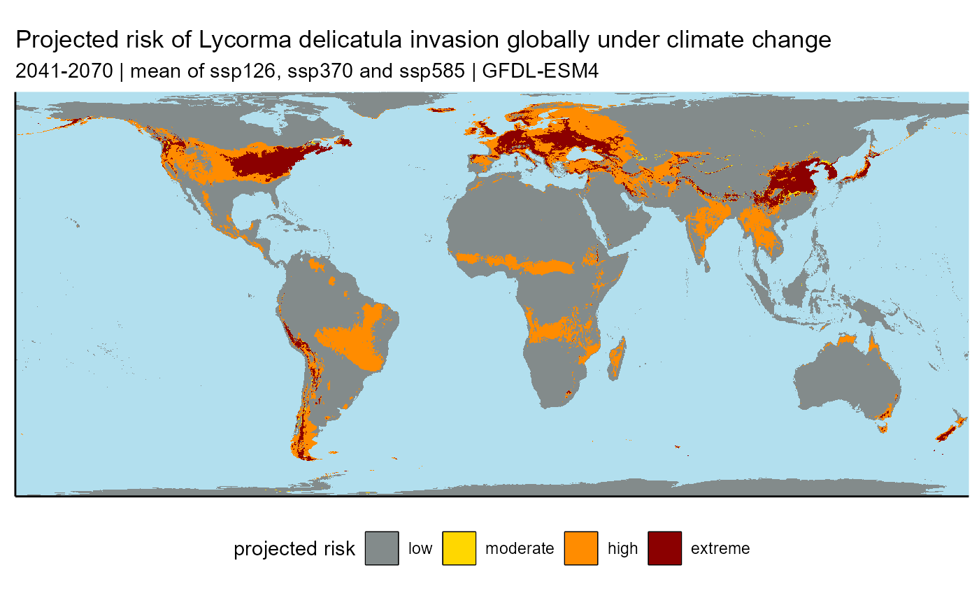
3. Calculate total area predicted by each model

The figures above are classified into categories of low, moderate, high and extreme risk for SLF establishment. In addition to visualizing them, I want to know the total predicted area in each category.

I will calculate the total suitable area predicted by each category and model.

As a reminder, the categories in these rasters are:

SLF suitability	raster value
Unsuitable Agreement	5
Suitable Agreement	10
unsuitable regional/suitable global	9
Suitable regional/unsuitable global	6

# load rasters
slf_binarized_1995 <- terra::rast(x = file.path(mypath, "working_dir", "slf_binarized_summed_1981-2010.asc")) 
slf_binarized_2055_ssp_mean <- terra::rast(x = file.path(mypath, "working_dir", "slf_binarized_summed_2041-2070_ssp_mean_GFDL.asc")) 

# 1995
slf_model_prop_table_1995 <- terra::expanse(
  x = slf_binarized_1995,
  unit = "km",
  byValue = TRUE
) 

# 2055
slf_model_prop_table_2055_ssp_mean <- terra::expanse(
  x = slf_binarized_2055_ssp_mean,
  unit = "km",
  byValue = TRUE
)

# create list of range shift values
categories.obj <- tibble(
  model_suitability = c("unsuitable_agreement", "regional", "global", "suitable_agreement"),
  value = c(5, 6, 9, 10)
)

# join
slf_model_prop_table_joined <- left_join(slf_model_prop_table_1995, slf_model_prop_table_2055_ssp_mean, by = c("value", "layer")) %>%
  # add labels
  left_join(., categories.obj, by = "value")

# tidy
slf_model_prop_table_joined <- slf_model_prop_table_joined %>%
  dplyr::select(-c(layer, value)) %>%
  dplyr::rename(
    "area_km_1995" = "area.x",
    "area_km_2055" = "area.y"
    ) %>%
  dplyr::mutate(
    # make proportions
    prop_total_area_1995 = scales::label_percent()(area_km_1995 / sum(area_km_1995)),
    prop_total_area_2055 = scales::label_percent()(area_km_2055 / sum(area_km_2055)),
    # change labels
    area_km_1995 = scales::label_comma()(area_km_1995),
    area_km_2055 = scales::label_comma()(area_km_2055)
    ) %>%
  dplyr::relocate(model_suitability, area_km_1995, prop_total_area_1995, area_km_2055, prop_total_area_2055) %>%
  dplyr::rename(
   "prop_area_present" = "prop_total_area_1995",
   "prop_area_2041-2070" = "prop_total_area_2055"
  )

# add superscript
colnames(slf_model_prop_table_joined)[2] <- paste0("area_km", common::supsc("2"), "_present")
colnames(slf_model_prop_table_joined)[4] <- paste0("area_km", common::supsc("2"), "_2041-2070")

# .html formatting
# format row colors
slf_model_prop_table_joined[1, 1] <- kableExtra::cell_spec(slf_model_prop_table_joined[1, 1], format = "html", bold = TRUE, color = "azure4")
slf_model_prop_table_joined[2, 1] <- kableExtra::cell_spec(slf_model_prop_table_joined[2, 1], format = "html", bold = TRUE, color = "darkorange")
slf_model_prop_table_joined[3, 1] <- kableExtra::cell_spec(slf_model_prop_table_joined[3, 1], format = "html", bold = TRUE, color = "gold")
slf_model_prop_table_joined[4, 1] <- kableExtra::cell_spec(slf_model_prop_table_joined[4, 1], format = "html", bold = TRUE, color = "darkred")

# convert to kable
slf_model_prop_kable <- knitr::kable(x = slf_model_prop_table_joined, format = "html", escape = FALSE) %>%
  kableExtra::kable_styling(bootstrap_options = "striped", full_width = TRUE)
  
print(slf_model_prop_kable)

## <table class="table table-striped" style="margin-left: auto; margin-right: auto;">
##  <thead>
##   <tr>
##    <th style="text-align:left;"> model_suitability </th>
##    <th style="text-align:left;"> area_km²_present </th>
##    <th style="text-align:left;"> prop_area_present </th>
##    <th style="text-align:left;"> area_km²_2041-2070 </th>
##    <th style="text-align:left;"> prop_area_2041-2070 </th>
##   </tr>
##  </thead>
## <tbody>
##   <tr>
##    <td style="text-align:left;"> <span style=" font-weight: bold;    color: rgba(131, 139, 139, 255) !important;">unsuitable_agreement</span> </td>
##    <td style="text-align:left;"> 118,348,996 </td>
##    <td style="text-align:left;"> 85.86% </td>
##    <td style="text-align:left;"> 117,048,301 </td>
##    <td style="text-align:left;"> 84.9% </td>
##   </tr>
##   <tr>
##    <td style="text-align:left;"> <span style=" font-weight: bold;    color: darkorange !important;">regional</span> </td>
##    <td style="text-align:left;"> 9,364,463 </td>
##    <td style="text-align:left;"> 6.79% </td>
##    <td style="text-align:left;"> 11,062,245 </td>
##    <td style="text-align:left;"> 8.0% </td>
##   </tr>
##   <tr>
##    <td style="text-align:left;"> <span style=" font-weight: bold;    color: gold !important;">global</span> </td>
##    <td style="text-align:left;"> 1,132,243 </td>
##    <td style="text-align:left;"> 0.82% </td>
##    <td style="text-align:left;"> 1,244,449 </td>
##    <td style="text-align:left;"> 0.9% </td>
##   </tr>
##   <tr>
##    <td style="text-align:left;"> <span style=" font-weight: bold;    color: darkred !important;">suitable_agreement</span> </td>
##    <td style="text-align:left;"> 9,000,778 </td>
##    <td style="text-align:left;"> 6.53% </td>
##    <td style="text-align:left;"> 8,491,485 </td>
##    <td style="text-align:left;"> 6.2% </td>
##   </tr>
## </tbody>
## </table>

# model training dataset
# save as .csv
write_csv(slf_model_prop_table_joined, file.path(here::here(), "vignette-outputs", "data-tables", "slf_binarized_summed_areas_table.csv"))

# save as .html
kableExtra::save_kable(
  slf_model_prop_kable, 
  file = file.path(here::here(), "vignette-outputs", "figures", "slf_binarized_summed_areas_table.html"),
  self_contained = TRUE,
  bs_theme = "simplex"
  )

# initialize webshot by 
# webshot::install_phantomjs()
# convert to jpg
webshot::webshot(
  url = file.path(here::here(), "vignette-outputs", "figures", "slf_binarized_summed_areas_table.html"),
  file = file.path(here::here(), "vignette-outputs", "figures", "slf_binarized_summed_areas_table.jpg"),
  zoom = 2
)

# remove html
file.remove(file.path(here::here(), "vignette-outputs", "figures", "slf_binarized_summed_areas_table.html"))

4. Map range shifting areas

Lastly, I want to create a map of areas where SLF range is expanding, contracting or remaining the same over time. I will binarize the rasters so that any point that is above the MTSS threshold on either model becomes one number and anything above the threshold becomes another. This will follow a slightly altered version of the methodology from step 2.

I will classify the cells as the following:

Raster and suitability	cloglog range	binary value	output value
Historical unsuitable	5	00000001	1
Historical suitable	6, 9 or 10	00000010	2
2041-2070 unsuitable	5	00000100	4
2041-2070 suitable	6, 9 or 10	00001000	8

By encoding the rasters into base-2, I have created only 4 possible values of the raster layers, which can be translated into 4 categories. I will also interpret these categories in terms of risk of SLF range expansion::

Suitability agreement	summed value	binary value	interpretation
Unsuitable Agreement	5	00000101	will stay unsuitable (no range shift)
Suitable Agreement	10	00001010	will stay suitable (no range shift)
unsuitable hist/suitable 2041-2070	9	00001001	will become SUITABLE in the future (range expansion)
Suitable hist/unsuitable 2041-2070	6	00000110	will become UNSUITABLE in the future (range contraction)

I will classify areas of unsuitability as gray, per usual. Areas where SLF remains the same will be white, areas where SLF is expanding will be green, and areas where SLF is contracting will be red.

First, I will load in the historical binarized raster (the intersection between the regional and global models) and classify it in preparation for this analysis. Then, I will intersect this raster with each of the predicted ssp rasters and the mean of those scenarios.

4.1 Setup

# 1995
slf_binarized_1995 <- terra::rast(x = file.path(mypath, "working_dir", "slf_binarized_summed_1981-2010.asc")) 
# rename values
names(slf_binarized_1995) <- "global_regional_binarized_1995"

# convert to df
slf_binarized_1995_df <- terra::as.data.frame(slf_binarized_1995, xy = TRUE)

I will also load some classification matrices for terra::classify(). These should not change between maps because we are classifying based on the time period, which does not change.

# create historical suitability value matrix for terra
classes_1995 <- data.frame(
  is = c(5, 6, 9, 10),
  becomes = c(strtoi(00000001, base = 2), strtoi(00000010, base = 2), strtoi(00000010, base = 2), strtoi(00000010, base = 2)) 
  # the strtoi function converts to base-2, becomes 1 and 2
)

# the class for all CMIP6 scenarios
classes_2055 <- data.frame(
  is = c(5, 6, 9, 10),
  becomes = c(strtoi(00000100, base = 2), strtoi(00001000, base = 2), strtoi(00001000, base = 2), strtoi(00001000, base = 2)) 
  # becomes 4 and 8
)

I will go ahead and classify the historical binarized raster because I will use it in the next steps

# reclassify and write the historical binarized raster
slf_binarized_1995_classified <- terra::classify(
  x = slf_binarized_1995, 
  rcl = classes_1995,
  others = strtoi(00000001, base = 2),
  filename = file.path(mypath, "working_dir", "slf_range_shift_1981-2010.asc"), # also write to file
  filetype = "AAIGrid",
  overwrite = FALSE
  )

I will quickly ensure that the binarization process worked by creating a rough plot.

# load in binary raster just created and convert to df
slf_binarized_1995_classified_df <- terra::rast(
  x = file.path(mypath, "working_dir", "slf_range_shift_1981-2010.asc")
  ) %>%
  terra::as.data.frame(., xy = TRUE) #%>%
  #na.omit()

# now, create vectors of values used to manually edit the scale of the plot
# the possible values of the scale and their order
breaks.obj <- unique(slf_binarized_1995_classified_df$global_regional_binarized_1995)
# labels for the values
labels.obj <- c("present unsuitable", "present suitable")
# vector of colors to classify scale
values.obj <- c(
  "azure4",
  "azure"
)

# plot regional binary
ggplot() +
  geom_raster(data = slf_binarized_1995_classified_df, aes(x = x, y = y, fill = as.factor(global_regional_binarized_1995))) +
  labs(title = "current suitability for SLF") +
  scale_fill_manual(
    name = "suitability for SLF",
    values = values.obj,
    breaks = breaks.obj,
    labels = labels.obj,
    aesthetics = "fill",
    ) +
  map_style_binarized

The conversion worked, as anything colorful on the binarized map should now be white. I will load a helper function for future plotting, similar to the one in step 2.2. I will interpret these categories in terms range shifts, as discussed above:

Unsuitable Agreement = 5 -> area will stay unsuitable (no range shift)
Suitable Agreement = 10 -> area will stay suitable (no range shift)
unsuitable 1995/suitable 2055 = 9 -> area will become SUITABLE in the future (range expansion)
Suitable 1995/unsuitable 2055 = 6 -> area will become UNSUITABLE in the future (range contraction)

# vectors of values used to manually edit the scale of the plot
# the possible values of the scale and their order
breaks.obj <- c(5, 10, 6, 9) # i manually ordered these according to the order produced from unique(slf_range_shift_126_df$range_shift_summed)
# labels for the values
labels.obj <- c("unsuitable area\nretained", "suitabile area\nretained", "contraction\nsuitable area", "expansion\nsuitable area")
# vector of colors to classify scale
values.obj <- c("azure4", "azure", "darkred", "darkgreen")


# function
plot_range_shift <- function(raster.df) {
  
  # raster.df = the df of the raster to be plotted
  
  ggplot() +
    # default style
    map_style_binarized +
    # plot raster
    geom_raster(data = raster.df, aes(x = x, y = y, fill = as.factor(range_shift_summed))) +
    # discretized scale 
    scale_discrete_manual(
      name = "L delicatula\nsuitability shift",
      values = values.obj, # the colors
      breaks = breaks.obj, # the breaks in the colors (4 since this is a discrete scale)
      labels = labels.obj, # the labels per color bin
      aesthetics = "fill",
      guide = guide_colorsteps(frame.colour = "black", ticks.colour = "black", barwidth = 20, draw.ulim = TRUE, draw.llim = TRUE)
      ) +
    # aesthetics
    guides(fill = guide_legend(nrow = 1, byrow = TRUE)) +
    theme(legend.key = element_rect(color = "black"), legend.title = element_text(hjust = 1)) 
  
}

I will create another helper function to format a range shift table per ssp scenario, which I will create later.

# create list of range shift values
ranges.obj <- c("remains_unsuitable", "contraction", "expansion", "retained_suitability")

table_range_shift <- function(table.df) {
  
  # table.df = dataframe of areas for raster bins, created by terra::expanse

  # tidy
  table.df.output <- table.df %>%
    dplyr::select(-layer) %>%
    dplyr::mutate(
      Ld_range_shift_type = ranges.obj,
      prop_total_area = scales::label_percent()(area / sum(area)),
      area = scales::label_comma()(area)
      ) %>%
    dplyr::select(-value) %>%
    dplyr::relocate(Ld_range_shift_type, area)
  
  colnames(table.df.output)[2] <- paste0("area_km", common::supsc("2"))
  
  
# .html formatting
# format row colors
table.df.output[1, 1] <- kableExtra::cell_spec(table.df.output[1, 1], format = "html", background = "azure4")
table.df.output[2, 1] <- kableExtra::cell_spec(table.df.output[2, 1], format = "html", background = "darkred")
table.df.output[3, 1] <- kableExtra::cell_spec(table.df.output[3, 1], format = "html", background = "darkgreen")
table.df.output[4, 1] <- kableExtra::cell_spec(table.df.output[4, 1], format = "html", background = "azure")
  

# return
return(table.df.output)

}

4.2 ssp 126

classify

slf_binarized_2055_126 <- terra::rast(x = file.path(mypath, "working_dir", "slf_binarized_summed_2041-2070_ssp126_GFDL.asc")) 
# rename values
names(slf_binarized_2055_126) <- "global_regional_binarized_2055_126"

# convert to df
slf_binarized_2055_126_df <- terra::as.data.frame(slf_binarized_2055_126, xy = TRUE)

unique(values(slf_binarized_1995))

unique(values(slf_binarized_2055_126))

# all looks good

# global
# reclassify and write binarized raster
slf_binarized_2055_126_classified <- terra::classify(
  x = slf_binarized_2055_126, 
  rcl = classes_2055, 
  others = strtoi(00000100, base = 2),
  filename = file.path(mypath, "working_dir", "slf_range_shift_2041-2070_ssp126_GFDL.asc"), 
  filetype = "AAIGrid",
  overwrite = FALSE
  )

I will run a few error checks to ensure that the binarization process worked.

# take minmax
terra::minmax(slf_binarized_1995_classified) %>%
  format(., scientific = FALSE)

terra::minmax(slf_binarized_2055_126_classified) %>%
  format(., scientific = FALSE)

# all good

# check unique values
unique(values(slf_binarized_1995_classified))
unique(values(slf_binarized_2055_126_classified))

Mosaic

Next, I will need to stack the reclassified 1995 and 2055 rasters and add them into a single raster output. This should give me the a raster with 4 classes:

Unsuitable Agreement = 5
Suitable Agreement = 10
unsuitable 1995/suitable 2055 = 9
Suitable 1995/unsuitable 2055 = 6

The mosaic function combines spatRasters that overlap in extent into a new raster, via the function specified (addition, in this case).

slf_binarized_1995_classified <- terra::rast(x = file.path(mypath, "working_dir", "slf_range_shift_1981-2010.asc"))

slf_binarized_2055_126_classified <- terra::rast(x = file.path(mypath, "working_dir", "slf_range_shift_2041-2070_ssp126_GFDL.asc"))

# overlay and combine rasters by summing values
slf_range_shift_126 <- terra::mosaic(
  slf_binarized_1995_classified, slf_binarized_2055_126_classified, # rasters
  fun = "sum", 
  filename = file.path(mypath, "working_dir", "slf_range_shift_summed_ssp126_GFDL.asc"),
  overwrite = FALSE,
  wopt = list(
    progress = 1,
    names = "range_shift_summed"
    )
  ) # progress bar

Plot

# re-load created raster
slf_range_shift_126 <- terra::rast(x = file.path(mypath, "working_dir", "slf_range_shift_summed_ssp126_GFDL.asc")) 
# convert to df
slf_range_shift_126_df <- terra::as.data.frame(slf_range_shift_126, xy = TRUE) #%>%
 # na.omit()

# check for the number of unique values in the raster values column
unique(slf_range_shift_126_df$range_shift_summed)

## [1]  5  9 10  6

# it seems that the reclassification worked! Lets map it to be sure.

slf_range_shift_126_plot <- plot_range_shift(
  raster.df = slf_range_shift_126_df
) +
  # labels
  labs(
    title = "Projected areas suitable for Lycorma delicatula range expansion",
    subtitle = "2041-2070 | ssp126 GFDL-ESM4"
    )

ggsave(
  slf_range_shift_126_plot, 
  filename = file.path(here::here(), "vignette-outputs", "figures", "slf_range_shift_summed_ssp126_GFDL.jpg"),
  height = 8, 
  width = 12,
  device = jpeg,
  dpi = "retina"
  )

sum areas gained and lost

slf_range_shift_126_table <- terra::expanse(
  x = slf_range_shift_126,
  unit = "km",
  byValue = TRUE
)

slf_range_shift_126_table <- table_range_shift(table.df = slf_range_shift_126_table)

# save as .csv
write_csv(slf_range_shift_126_table, file.path(here::here(), "vignette-outputs", "data-tables", "slf_range_shift_summed_area_table_ssp126_GFDL.csv"))

# convert to kable
slf_range_shift_126_kable <- knitr::kable(x = slf_range_shift_126_table, format = "html", escape = FALSE) %>%
  kableExtra::kable_styling(bootstrap_options = "striped", full_width = FALSE)

# save as .html
kableExtra::save_kable(
  slf_range_shift_126_kable, 
  file = file.path(here::here(), "vignette-outputs", "figures", "slf_range_shift_summed_area_table_ssp126_GFDL.html"),
  self_contained = TRUE,
  bs_theme = "simplex"
  )

# initialize webshot by 
# webshot::install_phantomjs()
# convert to pdf
webshot::webshot(
  url = file.path(here::here(), "vignette-outputs", "figures", "slf_range_shift_summed_area_table_ssp126_GFDL.html"),
  file = file.path(here::here(), "vignette-outputs", "figures", "slf_range_shift_summed_area_table_ssp126_GFDL.jpg"),
  zoom = 2
)

# remove .html
file.remove(file.path(here::here(), "vignette-outputs", "figures", "slf_range_shift_summed_area_table_ssp126_GFDL.html"))

Now, I will repeat this process for the other SSP scenarios and the mean of those scenarios (code not shown).

classify

slf_binarized_2055_370 <- terra::rast(x = file.path(mypath, "working_dir", "slf_binarized_summed_2041-2070_ssp370_GFDL.asc")) 
# rename values
names(slf_binarized_2055_370) <- "global_regional_binarized_2055_370"

# convert to df
slf_binarized_2055_370_df <- terra::as.data.frame(slf_binarized_2055_370, xy = TRUE)

unique(values(slf_binarized_1995))

unique(values(slf_binarized_2055_370))

# all looks good

# global
# reclassify and write global raster
slf_binarized_2055_370_classified <- terra::classify(
  x = slf_binarized_2055_370, 
  rcl = classes_2055, 
  others = strtoi(00000100, base = 2),
  filename = file.path(mypath, "working_dir", "slf_range_shift_2041-2070_ssp370_GFDL.asc"), 
  filetype = "AAIGrid",
  overwrite = FALSE
  )

I will run a few error checks to ensure that the binarization process worked.

# take minmax
terra::minmax(slf_binarized_1995_classified) %>%
  format(., scientific = FALSE)

terra::minmax(slf_binarized_2055_370_classified) %>%
  format(., scientific = FALSE)

# all good

# check unique values
unique(values(slf_binarized_1995_classified))
unique(values(slf_binarized_2055_370_classified))

Mosaic

slf_binarized_1995_classified <- terra::rast(x = file.path(mypath, "working_dir", "slf_range_shift_1981-2010.asc"))

slf_binarized_2055_370_classified <- terra::rast(x = file.path(mypath, "working_dir", "slf_range_shift_2041-2070_ssp370_GFDL.asc"))

# overlay and combine rasters by summing values
slf_range_shift_370 <- terra::mosaic(
  slf_binarized_1995_classified, slf_binarized_2055_370_classified, # rasters
  fun = "sum", 
  filename = file.path(mypath, "working_dir", "slf_range_shift_summed_ssp370_GFDL.asc"),
  overwrite = FALSE,
  wopt = list(
    progress = 1,
    names = "range_shift_summed"
    )
  ) # progress bar

Plot

# re-load created raster
slf_range_shift_370 <- terra::rast(x = file.path(mypath, "working_dir", "slf_range_shift_summed_ssp370_GFDL.asc")) 
# convert to df
slf_range_shift_370_df <- terra::as.data.frame(slf_range_shift_370, xy = TRUE) #%>%
 # na.omit()

# check for the number of unique values in the raster values column
unique(slf_range_shift_370_df$range_shift_summed)
# it seems that the reclassification worked! Lets map it to be sure.

slf_range_shift_370_plot <- plot_range_shift(
  raster.df = slf_range_shift_370_df
) +
  # labels
  labs(
    title = "Projected areas suitable for Lycorma delicatula range expansion",
    subtitle = "2041-2070 | ssp370 GFDL-ESM4"
    )

ggsave(
  slf_range_shift_370_plot, 
  filename = file.path(here::here(), "vignette-outputs", "figures", "slf_range_shift_summed_ssp370_GFDL.jpg"),
  height = 8, 
  width = 12,
  device = jpeg,
  dpi = "retina"
  )

sum areas gained and lost

slf_range_shift_370_table <- terra::expanse(
  x = slf_range_shift_370,
  unit = "km",
  byValue = TRUE
)

slf_range_shift_370_table <- table_range_shift(table.df = slf_range_shift_370_table)

# save as .csv
write_csv(slf_range_shift_370_table, file.path(here::here(), "vignette-outputs", "data-tables", "slf_range_shift_summed_area_table_ssp370_GFDL.csv"))

# convert to kable
slf_range_shift_370_kable <- knitr::kable(x = slf_range_shift_370_table, format = "html", escape = FALSE) %>%
  kableExtra::kable_styling(bootstrap_options = "striped", full_width = FALSE)

# save as .html
kableExtra::save_kable(
  slf_range_shift_370_kable, 
  file = file.path(here::here(), "vignette-outputs", "figures", "slf_range_shift_summed_area_table_ssp370_GFDL.html"),
  self_contained = TRUE,
  bs_theme = "simplex"
  )

# initialize webshot by 
# webshot::install_phantomjs()
# convert to pdf
webshot::webshot(
  url = file.path(here::here(), "vignette-outputs", "figures", "slf_range_shift_summed_area_table_ssp370_GFDL.html"),
  file = file.path(here::here(), "vignette-outputs", "figures", "slf_range_shift_summed_area_table_ssp370_GFDL.jpg"),
  zoom = 2
)

# remove .html
file.remove(file.path(here::here(), "vignette-outputs", "figures", "slf_range_shift_summed_area_table_ssp370_GFDL.html"))

classify

slf_binarized_2055_585 <- terra::rast(x = file.path(mypath, "working_dir", "slf_binarized_summed_2041-2070_ssp585_GFDL.asc")) 
# rename values
names(slf_binarized_2055_585) <- "global_regional_binarized_2055_585"

# convert to df
slf_binarized_2055_585_df <- terra::as.data.frame(slf_binarized_2055_585, xy = TRUE)

unique(values(slf_binarized_1995))

unique(values(slf_binarized_2055_585))

# all looks good

# global
# reclassify and write global raster
slf_binarized_2055_585_classified <- terra::classify(
  x = slf_binarized_2055_585, 
  rcl = classes_2055, 
  others = strtoi(00000100, base = 2),
  filename = file.path(mypath, "working_dir", "slf_range_shift_2041-2070_ssp585_GFDL.asc"), 
  filetype = "AAIGrid",
  overwrite = FALSE
  )

I will run a few error checks to ensure that the binarization process worked.

# take minmax
terra::minmax(slf_binarized_1995_classified) %>%
  format(., scientific = FALSE)

terra::minmax(slf_binarized_2055_585_classified) %>%
  format(., scientific = FALSE)

# all good

# check unique values
unique(values(slf_binarized_1995_classified))
unique(values(slf_binarized_2055_585_classified))

Mosaic

slf_binarized_1995_classified <- terra::rast(x = file.path(mypath, "working_dir", "slf_range_shift_1981-2010.asc"))

slf_binarized_2055_585_classified <- terra::rast(x = file.path(mypath, "working_dir", "slf_range_shift_2041-2070_ssp585_GFDL.asc"))

# overlay and combine rasters by summing values
slf_range_shift_585 <- terra::mosaic(
  slf_binarized_1995_classified, slf_binarized_2055_585_classified, # rasters
  fun = "sum", 
  filename = file.path(mypath, "working_dir", "slf_range_shift_summed_ssp585_GFDL.asc"),
  overwrite = FALSE,
  wopt = list(
    progress = 1,
    names = "range_shift_summed"
    )
  ) # progress bar

Plot

# re-load created raster
slf_range_shift_585 <- terra::rast(x = file.path(mypath, "working_dir", "slf_range_shift_summed_ssp585_GFDL.asc")) 
# convert to df
slf_range_shift_585_df <- terra::as.data.frame(slf_range_shift_585, xy = TRUE) #%>%
 # na.omit()

# check for the number of unique values in the raster values column
unique(slf_range_shift_585_df$range_shift_summed)
# it seems that the reclassification worked! Lets map it to be sure.

slf_range_shift_585_plot <- plot_range_shift(
  raster.df = slf_range_shift_585_df
) +
  # labels
  labs(
    title = "Projected areas suitable for Lycorma delicatula range expansion",
    subtitle = "2041-2070 | ssp585 GFDL-ESM4"
    )

ggsave(
  slf_range_shift_585_plot, 
  filename = file.path(here::here(), "vignette-outputs", "figures", "slf_range_shift_summed_ssp585_GFDL.jpg"),
  height = 8, 
  width = 12,
  device = jpeg,
  dpi = "retina"
  )

sum areas gained and lost

slf_range_shift_585_table <- terra::expanse(
  x = slf_range_shift_585,
  unit = "km",
  byValue = TRUE
)

slf_range_shift_585_table <- table_range_shift(table.df = slf_range_shift_585_table)

# save as .csv
write_csv(slf_range_shift_585_table, file.path(here::here(), "vignette-outputs", "data-tables", "slf_range_shift_summed_area_table_ssp585_GFDL.csv"))

# convert to kable
slf_range_shift_585_kable <- knitr::kable(x = slf_range_shift_585_table, format = "html", escape = FALSE) %>%
  kableExtra::kable_styling(bootstrap_options = "striped", full_width = FALSE)

# save as .html
kableExtra::save_kable(
  slf_range_shift_585_kable, 
  file = file.path(here::here(), "vignette-outputs", "figures", "slf_range_shift_summed_area_table_ssp585_GFDL.html"),
  self_contained = TRUE,
  bs_theme = "simplex"
  )

# initialize webshot by 
# webshot::install_phantomjs()
# convert to pdf
webshot::webshot(
  url = file.path(here::here(), "vignette-outputs", "figures", "slf_range_shift_summed_area_table_ssp585_GFDL.html"),
  file = file.path(here::here(), "vignette-outputs", "figures", "slf_range_shift_summed_area_table_ssp585_GFDL.jpg"),
  zoom = 2
)

# remove .html
file.remove(file.path(here::here(), "vignette-outputs", "figures", "slf_range_shift_summed_area_table_ssp585_GFDL.html"))

4.5 ssp ssp_mean

classify

slf_binarized_2055_ssp_mean <- terra::rast(x = file.path(mypath, "working_dir", "slf_binarized_summed_2041-2070_ssp_mean_GFDL.asc")) 
# rename values
names(slf_binarized_2055_ssp_mean) <- "global_regional_binarized_2055_ssp_mean"

# convert to df
slf_binarized_2055_ssp_mean_df <- terra::as.data.frame(slf_binarized_2055_ssp_mean, xy = TRUE)

unique(values(slf_binarized_1995))

unique(values(slf_binarized_2055_ssp_mean))

# all looks good

# global
# reclassify and write global raster
slf_binarized_2055_ssp_mean_classified <- terra::classify(
  x = slf_binarized_2055_ssp_mean, 
  rcl = classes_2055, 
  others = strtoi(00000100, base = 2),
  filename = file.path(mypath, "working_dir", "slf_range_shift_2041-2070_ssp_mean_GFDL.asc"), 
  filetype = "AAIGrid",
  overwrite = FALSE
  )

I will run a few error checks to ensure that the binarization process worked.

# take minmax
terra::minmax(slf_binarized_1995_classified) %>%
  format(., scientific = FALSE)

terra::minmax(slf_binarized_2055_ssp_mean_classified) %>%
  format(., scientific = FALSE)

# all good

# check unique values
unique(values(slf_binarized_1995_classified))
unique(values(slf_binarized_2055_ssp_mean_classified))

Mosaic

slf_binarized_1995_classified <- terra::rast(x = file.path(mypath, "working_dir", "slf_range_shift_1981-2010.asc"))

slf_binarized_2055_ssp_mean_classified <- terra::rast(x = file.path(mypath, "working_dir", "slf_range_shift_2041-2070_ssp_mean_GFDL.asc"))

# overlay and combine rasters by summing values
slf_range_shift_ssp_mean <- terra::mosaic(
  slf_binarized_1995_classified, slf_binarized_2055_ssp_mean_classified, # rasters
  fun = "sum", 
  filename = file.path(mypath, "working_dir", "slf_range_shift_summed_ssp_mean_GFDL.asc"),
  overwrite = FALSE,
  wopt = list(
    progress = 1,
    names = "range_shift_summed"
    )
  ) # progress bar

Plot

# re-load created raster
slf_range_shift_ssp_mean <- terra::rast(x = file.path(mypath, "working_dir", "slf_range_shift_summed_ssp_mean_GFDL.asc")) 
# convert to df
slf_range_shift_ssp_mean_df <- terra::as.data.frame(slf_range_shift_ssp_mean, xy = TRUE) #%>%
 # na.omit()

# check for the number of unique values in the raster values column
unique(slf_range_shift_ssp_mean_df$range_shift_summed)

## [1]  5  9 10  6

# it seems that the reclassification worked! Lets map it to be sure.

slf_range_shift_ssp_mean_plot <- plot_range_shift(
  raster.df = slf_range_shift_ssp_mean_df
) +
  # labels
  labs(
    title = "Projected areas suitable for Lycorma delicatula range expansion",
    subtitle = "2041-2070 | mean of ssp126, ssp370 and ssp585, GFDL-ESM4"
    )

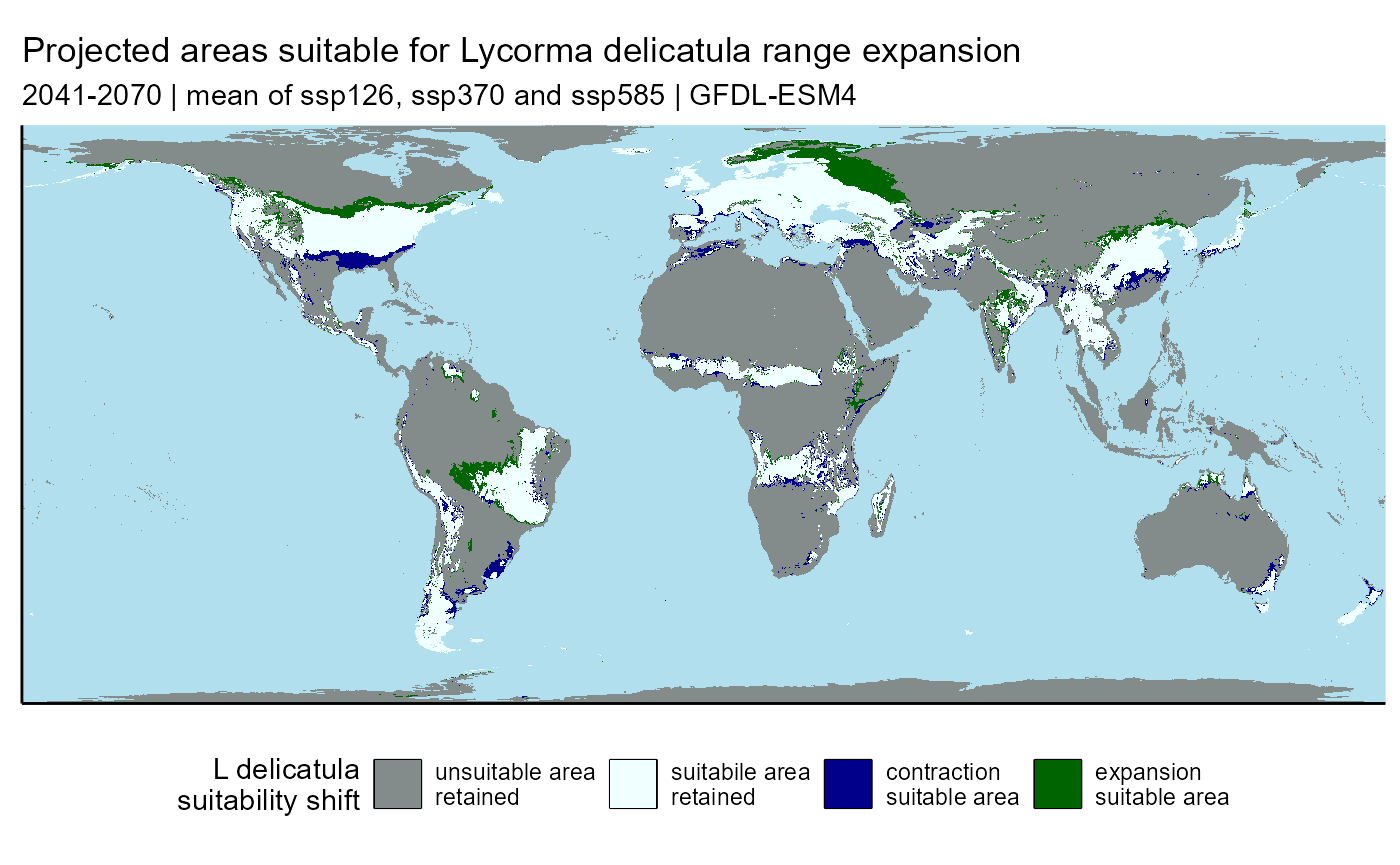
ggsave(
  slf_range_shift_ssp_mean_plot, 
  filename = file.path(here::here(), "vignette-outputs", "figures", "slf_range_shift_summed_ssp_mean_GFDL.jpg"),
  height = 8, 
  width = 12,
  device = jpeg,
  dpi = "retina"
  )

sum areas gained and lost

slf_range_shift_ssp_mean_table <- terra::expanse(
  x = slf_range_shift_ssp_mean,
  unit = "km",
  byValue = TRUE
)

slf_range_shift_ssp_mean_table <- table_range_shift(table.df = slf_range_shift_ssp_mean_table, eval = TRUE)

# save as .csv
write_csv(slf_range_shift_ssp_mean_table, file.path(here::here(), "vignette-outputs", "data-tables", "slf_range_shift_summed_area_table_ssp_mean_GFDL.csv"))

# convert to kable
slf_range_shift_ssp_mean_kable <- knitr::kable(x = slf_range_shift_ssp_mean_table, format = "html", escape = FALSE) %>%
  kableExtra::kable_styling(bootstrap_options = "striped", full_width = FALSE)

# save as .html
kableExtra::save_kable(
  slf_range_shift_ssp_mean_kable, 
  file = file.path(here::here(), "vignette-outputs", "figures", "slf_range_shift_summed_area_table_ssp_mean_GFDL.html"),
  self_contained = TRUE,
  bs_theme = "simplex"
  )

# initialize webshot by 
# webshot::install_phantomjs()
# convert to pdf
webshot::webshot(
  url = file.path(here::here(), "vignette-outputs", "figures", "slf_range_shift_summed_area_table_ssp_mean_GFDL.html"),
  file = file.path(here::here(), "vignette-outputs", "figures", "slf_range_shift_summed_area_table_ssp_mean_GFDL.jpg"),
  zoom = 2
)

# remove .html
file.remove(file.path(here::here(), "vignette-outputs", "figures", "slf_range_shift_summed_area_table_ssp_mean_GFDL.html"))

References

Gallien, L., Douzet, R., Pratte, S., Zimmermann, N. E., & Thuiller, W. (2012). Invasive species distribution models – how violating the equilibrium assumption can create new insights. Global Ecology and Biogeography, 21(11), 1126–1136. https://doi.org/10.1111/j.1466-8238.2012.00768.x
Liu, C., White, M., & Newell, G. (2013). Selecting thresholds for the prediction of species occurrence with presence-only data. Journal of Biogeography, 40(4), 778–789. https://doi.org/10.1111/jbi.12058
Liu, C., Newell, G., & White, M. (2016). On the selection of thresholds for predicting species occurrence with presence-only data. Ecology and Evolution, 6(1), 337–348. https://doi.org/10.1002/ece3.1878

Add country admin boundaries to risk plots

# load data
global_countries <- sf::st_read(dsn = file.path(here::here(), "data-raw", "ne_countries", "ne_10m_admin_0_countries.shp"))

1995

# plot
slf_binarized_1995_plot_withCountries <- slf_binarized_1995_plot +
  geom_sf(data = global_countries, aes(geometry = geometry), fill = NA, color = "black", linewidth = 0.15) + 
  # re-crop to usual boundaries
  coord_sf(xlim = c(-180.00013888885, 178.999859675084), ylim = c(-58.5001390148238, 82.99986041915))

# save
ggsave(
  slf_binarized_1995_plot_withCountries, 
  filename = file.path(here::here(), "vignette-outputs", "figures", "slf_binarized_summed_countries_1981-2010.jpg"),
  height = 8, 
  width = 12,
  device = jpeg,
  dpi = "retina"
  )

2055

For this analysis, I will only plot the raster of the mean of the 3 ssp scenarios.

# plot
slf_binarized_2055_plot_withCountries <- slf_binarized_2055_ssp_mean_plot +
  geom_sf(data = global_countries, aes(geometry = geometry), fill = NA, color = "black", linewidth = 0.15) + 
  # re-crop to usual boundaries
  coord_sf(xlim = c(-180.00013888885, 178.999859675084), ylim = c(-58.5001390148238, 82.99986041915))


# save
ggsave(
  slf_binarized_2055_plot_withCountries, 
  filename = file.path(here::here(), "vignette-outputs", "figures", "slf_binarized_summed_countries_2041-2070_ssp_mean_GFDL.jpg"),
  height = 8, 
  width = 12,
  device = jpeg,
  dpi = "retina"
  )

create patchwork of risk plots

slf_binarized_1995_plot_withCountries <- slf_binarized_1995_plot_withCountries + 
  theme(
    plot.title = element_blank(),
    plot.subtitle = element_blank(),
    plot.caption = element_blank(),
    axis.title = element_blank(),
    plot.tag.location = "panel",
    plot.tag.position = c(0.05, 0.1),
    plot.tag = element_text(face = "bold", size = 20),
    legend.title = element_text(face = "bold")
    ) +
  labs(tag = "A") +
  scale_x_continuous(expand = c(0, 0)) +
  scale_y_continuous(expand = c(0, 0)) 


slf_binarized_2055_plot_withCountries <- slf_binarized_2055_plot_withCountries + 
  theme(
    plot.title = element_blank(),
    plot.subtitle = element_blank(),
    plot.caption = element_blank(),
    axis.title = element_blank(),
    plot.tag.location = "panel",
    plot.tag.position = c(0.05, 0.1),
    plot.tag = element_text(face = "bold", size = 20),
    legend.title = element_text(face = "bold")
    ) +
  labs(tag = "B") +
  scale_x_continuous(expand = c(0, 0)) +
  scale_y_continuous(expand = c(0, 0)) 




slf_binarized_patchwork <- (slf_binarized_1995_plot_withCountries / slf_binarized_2055_plot_withCountries) +
  plot_annotation(
    title = "Projected risk of Lycorma delicatula invasion globally under climate change",
    subtitle = "(A) 1981-2010 (B) 2041-2070 | mean of ssp126, ssp370 and ssp85, GFDL-ESM4"
    ) +
  plot_layout(axes = "collect", guides = "collect") & 
  theme(legend.position = "bottom") 
  
  #plot_layout(widths = unit(20, "cm"))

ggsave(
  slf_binarized_patchwork, 
  filename = file.path(here::here(), "vignette-outputs", "figures", "slf_binarized_risk_patchwork_ssp_mean.jpg"),
  height = 8, 
  width = 12,
  device = jpeg,
  dpi = "retina"
  )

Samuel M. Owens1

2024-08-14

Overview

Setup

Import datasets

regional ensemble

Global model

1. Map cloglog suitability

1.1 Mapping helper function

1.2 Map cloglog output of models- historical

1.3 Map cloglog output of models- CMIP6

ssp mean

2. Create binary threshold maps to infer range filling

2.1 convert output rasters to binary predictors

historical

helper function- terra classify

ssp 126

ssp 370

ssp 585

ssp mean

2.2 Mosaic rasters and produce map

historical

helper function- binary raster plotting

ssp126

ssp370

ssp585

ssp mean

3. Calculate total area predicted by each model

4. Map range shifting areas

4.1 Setup

4.2 ssp 126

classify

Mosaic

Plot

sum areas gained and lost

4.3 ssp 370

4.4 ssp 585

4.5 ssp ssp_mean

References

Appendix

Add country admin boundaries to risk plots

1995

2055

create patchwork of risk plots

Samuel M. Owens¹