Infer stability of known SLF populations due climate change effects

Overview

In the last vignette, I created figures to analyze the suitability for SLF establishment at key viticultural regions globally. I will now apply this same framework to analyze the risk of establishment for currently known SLF populations. We will use this to infer the stability of these populations under climate change. We will use the same quadrant plot framework as in the last vignette.

## ── Attaching core tidyverse packages ──────────────────────── tidyverse 2.0.0 ──
## ✔ dplyr     1.1.4     ✔ readr     2.1.5
## ✔ forcats   1.0.0     ✔ stringr   1.5.1
## ✔ ggplot2   3.5.1     ✔ tibble    3.2.1
## ✔ lubridate 1.9.3     ✔ tidyr     1.3.1
## ✔ purrr     1.0.2     
## ── Conflicts ────────────────────────────────────────── tidyverse_conflicts() ──
## ✖ dplyr::filter() masks stats::filter()
## ✖ dplyr::lag()    masks stats::lag()
## ℹ Use the conflicted package (<http://conflicted.r-lib.org/>) to force all conflicts to become errors

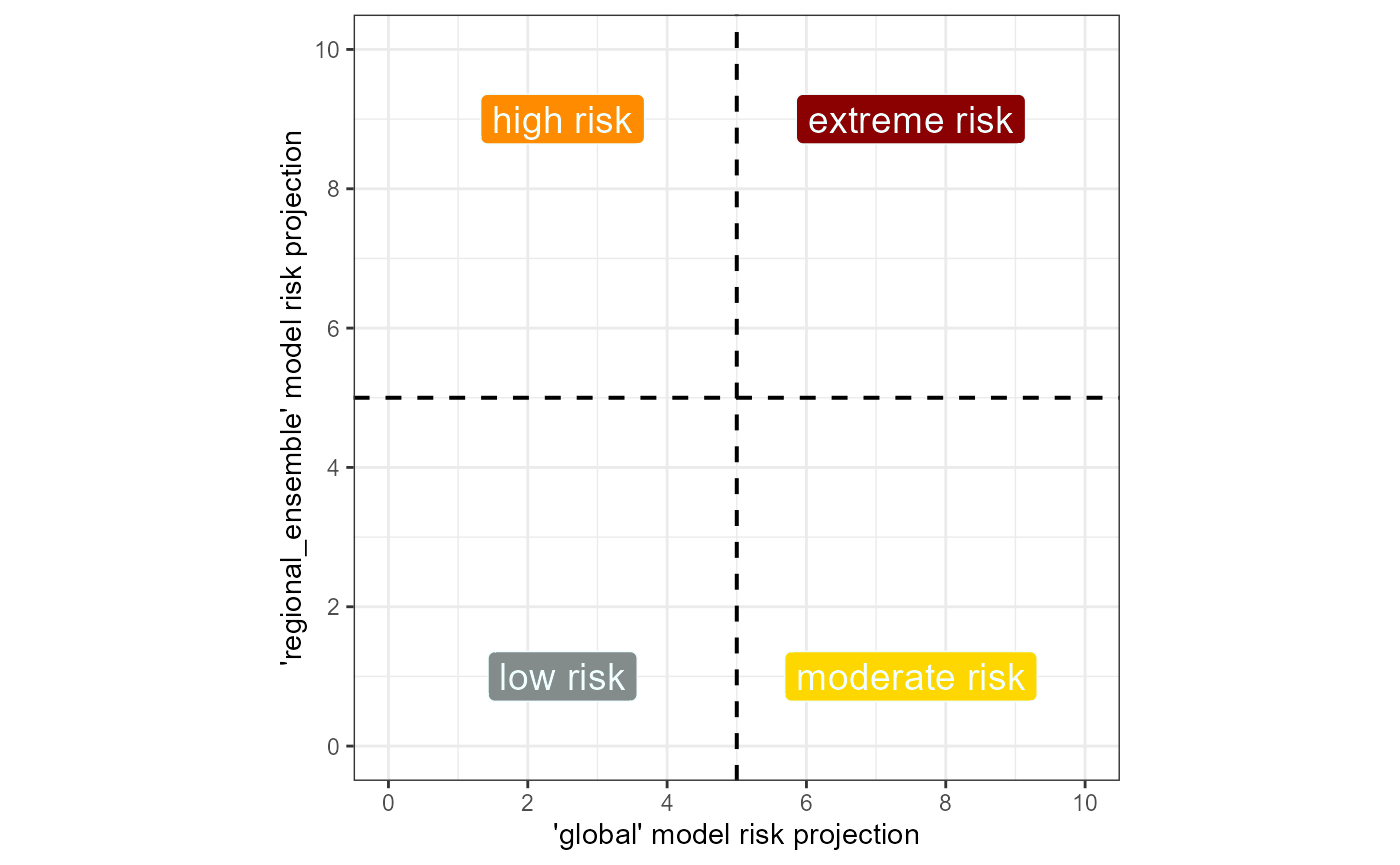Fig. 1 Example quadrant plot for assessing SLF risk across two different scales of SDM.

Setup

# general tools
library(tidyverse)  #data manipulation
library(here) #making directory pathways easier on different instances
# here() starts at the root folder of this package.
library(devtools)

# spatial data handling
library(terra)
library(CoordinateCleaner)

# plot aesthetics
library(scales)
library(patchwork)
library(grid)
library(kableExtra)
library(webshot)
library(webshot2)

Note: I will be setting the global options of this document so that only certain code chunks are rendered in the final .html file. I will set the eval = FALSE so that none of the code is re-run (preventing files from being overwritten during knitting) and will simply overwrite this in chunks with plots.

mypath <- file.path(here::here() %>% 
                       dirname(),
                     "maxent/models")

I will load in some aesthetic objects, including for breaks.

breaks <- c(0.0, 0.2, 0.4, 0.6, 0.8, 1.0)

labels <- c(0, 2, 4, 6, 8, 10)

Load in summary files for the global and regional ensemble models, which contain the thresholds.

# summary file to extract thresholds from

# global
summary_global <- read_csv(file = file.path(mypath, "slf_global_v3", "global_summary_all_iterations.csv"))

## Rows: 52 Columns: 12
## ── Column specification ────────────────────────────────────────────────────────
## Delimiter: ","
## chr  (1): statistic
## dbl (11): iteration_1_summary, iteration_2_summary, iteration_3_summary, ite...
## 
## ℹ Use `spec()` to retrieve the full column specification for this data.
## ℹ Specify the column types or set `show_col_types = FALSE` to quiet this message.

summary_regional_ensemble <- read_csv(file = file.path(mypath, "slf_regional_ensemble_v1", "ensemble_threshold_values.csv"))

## Rows: 10 Columns: 4
## ── Column specification ────────────────────────────────────────────────────────
## Delimiter: ","
## chr (3): thresh, time_period, CMIP6_model
## dbl (1): value
## 
## ℹ Use `spec()` to retrieve the full column specification for this data.
## ℹ Specify the column types or set `show_col_types = FALSE` to quiet this message.

load rasters

Finally, I will load in the global and regional ensemble suitability maps. These will be used both for extracting the new xy suitability values and for plotting.

# global
global_1995 <- terra::rast(x = file.path(mypath, "slf_global_v3", "global_pred_suit_clamped_cloglog_globe_1981-2010_mean.asc"))

global_2055 <- terra::rast(x = file.path(mypath, "slf_global_v3", "global_pred_suit_clamped_cloglog_globe_2041-2070_GFDL_ssp_averaged.asc"))


# regional_ensemble
# historical
regional_ensemble_1995 <- terra::rast(
  x = file.path(mypath, "slf_regional_ensemble_v1", "ensemble_regional_weighted_mean_globe_1981-2010.asc")
  )
# CMIP6
## ssp 126
regional_ensemble_2055_126 <- terra::rast(
  x = file.path(mypath, "slf_regional_ensemble_v1", "ensemble_regional_weighted_mean_globe_2041-2070_GFDL_ssp126.asc")
  )
# ssp 370
regional_ensemble_2055_370 <- terra::rast(
  x = file.path(mypath, "slf_regional_ensemble_v1", "ensemble_regional_weighted_mean_globe_2041-2070_GFDL_ssp370.asc")
  )
# ssp 585
regional_ensemble_2055_585 <- terra::rast(
  x = file.path(mypath, "slf_regional_ensemble_v1", "ensemble_regional_weighted_mean_globe_2041-2070_GFDL_ssp585.asc")
  )
# ssp mean
regional_ensemble_2055_ssp_mean <- terra::rast(
  x = file.path(mypath, "slf_regional_ensemble_v1", "ensemble_regional_weighted_mean_globe_2041-2070_GFDL_ssp_averaged.asc")
  )

tidy slf populations dataset

I will load in the dataset containing SLF populations.

slf_populations <- read_rds(file = file.path(here::here(), "data", "slf_all_coords_final_2024-08-05.rds"))

I will take steps to de-duplicate the slf populations dataset before retrieving suitability values for it.

slf_populations <- slf_populations %>%
  # filter out NAs
  dplyr::filter(
    !is.na(x),
    !is.na(y)
    ) %>% 
  # remove duplicate coordinates
  CoordinateCleaner::clean_coordinates(
    x = .,
    lon = "x",
    lat = "y",
    species = "species",
    tests = "duplicates",
    value = "clean" # just return same df without duplicates
  )

I will load in one of the xy_suitability files to compare with the slf populations dataset because some points were lost in the predict step, so now the slf populations dataset has more data points than the xy_suitability versions.

# historical
xy_global_1995 <- read_csv(
  file = file.path(mypath, "slf_global_v3", "global_slf_all_coords_1981-2010_xy_pred_suit_clamped_cloglog_mean.csv")
  )

# de-duplicate just to make sure
xy_global_1995 <- xy_global_1995 %>%
  CoordinateCleaner::clean_coordinates(
    x = .,
    lon = "x",
    lat = "y",
    species = "Species",
    tests = "duplicates",
    value = "clean"
  ) %>%
  dplyr::select(x, y, cloglog_suitability) %>%
  # rename
  dplyr::rename("cloglog_suit_hist" = "cloglog_suitability") 

# filter join of populations dataset
slf_populations <- semi_join(slf_populations, xy_global_1995, by = c("x", "y")) 
# add ID column
slf_populations <- slf_populations %>%
  dplyr::mutate(ID = row_number()) %>%
  relocate(ID)

Now that the records have been harmonized between the datasets, I will save to file for use downstream. This will be the main file for predicting slf population suitability.

if (FALSE) {

  readr::write_rds(slf_populations, file.path(here::here(), "data", "slf_all_coords_final_2024-08-05_tidied.rds"))
  
}

#read it back in
slf_populations <- read_rds(file.path(here::here(), "data", "slf_all_coords_final_2024-08-05_tidied.rds"))

import and tidy xy suitability

These scatter plots will be based on the suitability for the IVR points in both the global and regional_ensemble models. I have already calculated the xy suitability for the global model based on these points, using the function scari::predict_xy_suitability(). This function will not work for the regional_ensemble because it calls for a model object, which we did not use to predict the ensemble suitability. So, I will use terra::extract() to perform this action.

I will load in the global model datasets and create the regional_ensemble datasets. I will also do some tidying of my datasets for the plots I will create.

# CMIP6
## ssp 126
xy_global_2055_126 <- read_csv(
  file = file.path(mypath, "slf_global_v3", "global_slf_all_coords_2041-2070_GFDL_ssp126_xy_pred_suit_clamped_cloglog_mean.csv")
  ) 
## ssp 370
xy_global_2055_370 <- read_csv(
  file = file.path(mypath, "slf_global_v3", "global_slf_all_coords_2041-2070_GFDL_ssp370_xy_pred_suit_clamped_cloglog_mean.csv")
  ) 
## ssp 585
xy_global_2055_585 <- read_csv(
  file = file.path(mypath, "slf_global_v3", "global_slf_all_coords_2041-2070_GFDL_ssp585_xy_pred_suit_clamped_cloglog_mean.csv")
  )

# ssp 126
xy_global_2055_126 <- xy_global_2055_126 %>%
  CoordinateCleaner::clean_coordinates(
    x = .,
    lon = "x",
    lat = "y",
    species = "Species",
    tests = "duplicates",
    value = "clean"
  ) %>%
  # tidy
  dplyr::select(-Species) %>%
  dplyr::rename("cloglog_suit_ssp126" = "cloglog_suitability") 

# ssp 370
xy_global_2055_370 <- xy_global_2055_370 %>%
  CoordinateCleaner::clean_coordinates(
    x = .,
    lon = "x",
    lat = "y",
    species = "Species",
    tests = "duplicates",
    value = "clean"
  ) %>%
  # tidy
  dplyr::select(-Species) %>%
  dplyr::rename("cloglog_suit_ssp370" = "cloglog_suitability") 

# ssp 585
xy_global_2055_585 <- xy_global_2055_585 %>%
  CoordinateCleaner::clean_coordinates(
    x = .,
    lon = "x",
    lat = "y",
    species = "Species",
    tests = "duplicates",
    value = "clean"
  ) %>%
  # tidy
  dplyr::select(-Species) %>%
  dplyr::rename("cloglog_suit_ssp585" = "cloglog_suitability")

take mean of global model ssp scenarios

I will take the mean of the suitability value within each of these predicted suitability datasets to create a single prediction for the three ssp scenarios.

# first join datasets
xy_global_2055_ssp_mean <- xy_global_2055_126 %>%
  left_join(., xy_global_2055_370, join_by(x, y)) %>%
  left_join(., xy_global_2055_585, join_by(x, y)) %>%
  # take mean of columns
  dplyr::mutate(suit_ssp_averaged = rowMeans(.[, 3:5])) %>%
  dplyr::select(x, y, suit_ssp_averaged)

write_csv(
  x = xy_global_2055_ssp_mean,
  file = file.path(mypath, "slf_global_v3", "global_slf_all_coords_2041-2070_GFDL_ssp_mean_xy_pred_suit_clamped_cloglog_mean.csv")
    )

retrieve suitability values for regional_ensemble

Now, I will retrieve the suitability values for the regional_ensemble. Instead of returning the coordinates from the map, I will join the coordinates from the original slf_populations dataset so that the coordinates are exact for joining with other datasets. This step is much simpler than in the last vignette because I will be using a simple point-wise prediction method, instead of the buffer method used on the wineries datasets, as these coordinates represent exact population locations, rather than the centroid of a region.

# 1995
xy_regional_ensemble_1995 <- terra::extract(
  x = regional_ensemble_1995,
  y = dplyr::select(slf_populations, x, y), # points
  method = "simple",
  xy = FALSE, # dont return coordinates
  ID = TRUE
)

# CMIP6
# ssp126
xy_regional_ensemble_2055_126 <- terra::extract(
  x = regional_ensemble_2055_126,
  y = dplyr::select(slf_populations, x, y), # points
  method = "simple",
  xy = FALSE, # dont return coordinates 
  ID = TRUE
) 
# ssp370
xy_regional_ensemble_2055_370 <- terra::extract(
  x = regional_ensemble_2055_370,
  y = dplyr::select(slf_populations, x, y), # points
  method = "simple",
  xy = FALSE, # dont return coordinates 
  ID = TRUE
) 
# ssp126
xy_regional_ensemble_2055_585 <- terra::extract(
  x = regional_ensemble_2055_585,
  y = dplyr::select(slf_populations, x, y), # points
  method = "simple",
  xy = FALSE, # dont return coordinates 
  ID = TRUE
)

# joining object
slf_coordinates <- dplyr::select(slf_populations, ID, x, y)

# perform join
xy_regional_ensemble_1995 <- left_join(xy_regional_ensemble_1995, slf_coordinates, by = "ID") %>% 
  # tidy
  dplyr::relocate(ID, x, y) %>%
  dplyr::rename("cloglog_suit_hist" = "sum")
# CMIP6
## ssp 126
xy_regional_ensemble_2055_126 <- left_join(xy_regional_ensemble_2055_126, slf_coordinates, by = "ID") %>%
  dplyr::relocate(ID, x, y) %>%
  dplyr::rename("cloglog_suit_ssp126" = "sum")
## ssp370
xy_regional_ensemble_2055_370 <- left_join(xy_regional_ensemble_2055_370, slf_coordinates, by = "ID") %>%
  dplyr::relocate(ID, x, y) %>%
  dplyr::rename("cloglog_suit_ssp370" = "sum")
## ssp 585
xy_regional_ensemble_2055_585 <- left_join(xy_regional_ensemble_2055_585, slf_coordinates, by = "ID") %>%
  dplyr::relocate(ID, x, y) %>%
  dplyr::rename("cloglog_suit_ssp585" = "sum")

take mean of ssps

# first join datasets
xy_regional_ensemble_2055_ssp_mean <- xy_regional_ensemble_2055_126 %>%
  left_join(., xy_regional_ensemble_2055_370, join_by(ID, x, y)) %>%
  left_join(., xy_regional_ensemble_2055_585, join_by(ID, x, y)) %>%
  # take mean of columns
  dplyr::mutate(suit_ssp_averaged = rowMeans(.[, 4:6])) %>%
  dplyr::select(ID, x, y, suit_ssp_averaged)

write_csv(
  x = xy_regional_ensemble_2055_ssp_mean,
  file = file.path(mypath, "slf_regional_ensemble_v1", "regional_ensemble_wineries_2041-2070_GFDL_ssp_mean_xy_pred_suit.csv")
  )

write to file

Now, I will tidy and save the datasets to .rds for our analysis.

# global model datasets
xy_global_1995 <- xy_global_1995 %>%
  # add ID column
  cbind(., slf_populations[, 1]) %>%
  # rename the column for future joining
  dplyr::rename(
    "ID" = "slf_populations[, 1]",
    "xy_global_1995" = "cloglog_suit_hist"
    ) %>%
  dplyr::relocate(ID) 

  
xy_global_2055_ssp_mean <- xy_global_2055_ssp_mean %>%
  # add ID column
  cbind(., slf_populations[, 1]) %>%
  dplyr::rename(
    "ID" = "slf_populations[, 1]",
    "xy_global_2055" = "suit_ssp_averaged"
    ) %>%
  dplyr::relocate(ID)



# regional_ensemble datasets
xy_regional_ensemble_1995 <- xy_regional_ensemble_1995 %>%
  # rename the column for future joining
  dplyr::rename("xy_regional_ensemble_1995" = "cloglog_suit_hist") 

xy_regional_ensemble_2055_ssp_mean <- xy_regional_ensemble_2055_ssp_mean %>%
  # rename the column for future joining
  dplyr::rename("xy_regional_ensemble_2055" = "suit_ssp_averaged")

# save global datasets
readr::write_rds(
  xy_global_1995,  
  file = file.path(here::here(), "data", "global_slf_all_coords_1981-2010_xy_pred_suit.rds")
  )

readr::write_rds(
  xy_global_2055_ssp_mean,  
  file = file.path(here::here(), "data", "global_slf_all_coords_2041-2070_GFDL_ssp_mean_xy_pred_suit.rds")
  )


# regional_ensemble
readr::write_rds(
  xy_regional_ensemble_1995,  
  file = file.path(here::here(), "data", "regional_ensemble_slf_all_coords_1981-2010_xy_pred_suit.rds")
  )

readr::write_rds(
  xy_regional_ensemble_2055_ssp_mean,  
  file = file.path(here::here(), "data", "regional_ensemble_slf_all_coords_2041-2070_GFDL_ssp_mean_xy_pred_suit.rds")
  )

1. Transform xy suitability

I will plot the suitability values in two different ways- I will plot the raw xy suitability and I will transform the data so that the MTSS threshold is the center of the scatter plot. This way, movement across the minimum suitability threshold is more easily visualized. I will transform all 4 vectors of suitability values, 2 per model, in preparation for plotting.

I created the function scari::rescale_cloglog_suitability() to accomplish this task. This function uses a vector of exponential transformations for the specified value of thresh to apply an exponential equation to the vector of suitability values. It then applies the equation y = c1 * c2^x + c3 to the vector, where x is the input suitability values, y is the transformed version of those values, c1 and c3 are the maximum and its inverse, and c2 is the interpolated value of the input thresh. The transformed suitability vector is re-scaled so that thresh is the median (0.5) on a 0-1 scale and all other values are transformed to fit this scale.

slf_populations <- read_rds(file.path(here::here(), "data", "slf_all_coords_final_2024-08-05_tidied.rds"))

# global
xy_global_1995 <- read_rds(file = file.path(here::here(), "data", "global_slf_all_coords_1981-2010_xy_pred_suit.rds"))
xy_global_2055 <- read_rds(file = file.path(here::here(), "data", "global_slf_all_coords_2041-2070_GFDL_ssp_mean_xy_pred_suit.rds"))

# regional
xy_regional_ensemble_1995 <- read_rds(file = file.path(here::here(), "data", "regional_ensemble_slf_all_coords_1981-2010_xy_pred_suit.rds"))
xy_regional_ensemble_2055 <- read_rds(file = file.path(here::here(), "data", "regional_ensemble_slf_all_coords_2041-2070_GFDL_ssp_mean_xy_pred_suit.rds"))

xy_global_1995_rescaled <- scari::rescale_cloglog_suitability(
  xy.predicted = xy_global_1995,
  thresh = "MTSS",
  exponential.file = file.path(here::here(), "data-raw", "threshold_exponential_values.csv"),
  summary.file = summary_global,
  rescale.name = "xy_global_1995",
  rescale.thresholds = TRUE
)
# separate data from thresholds
xy_global_1995_rescaled_thresholds <- xy_global_1995_rescaled[[2]]
xy_global_1995_rescaled <- xy_global_1995_rescaled[[1]]



xy_global_2055_rescaled <- scari::rescale_cloglog_suitability(
  xy.predicted = xy_global_2055,
  thresh = "MTSS",  # the global model only has 1 MTSS thresh
  exponential.file = file.path(here::here(), "data-raw", "threshold_exponential_values.csv"),
  summary.file = summary_global,
  rescale.name = "xy_global_2055",
  rescale.thresholds = TRUE
)

xy_global_2055_rescaled_thresholds <- xy_global_2055_rescaled[[2]]
xy_global_2055_rescaled <- xy_global_2055_rescaled[[1]]

xy_regional_ensemble_1995_rescaled <- scari::rescale_cloglog_suitability(
  xy.predicted = xy_regional_ensemble_1995,
  thresh = "MTSS",
  exponential.file = file.path(here::here(), "data-raw", "threshold_exponential_values.csv"),
  summary.file = summary_regional_ensemble,
  rescale.name = "xy_regional_ensemble_1995",
  rescale.thresholds = TRUE
)

xy_regional_ensemble_1995_rescaled_thresholds <- xy_regional_ensemble_1995_rescaled[[2]]
xy_regional_ensemble_1995_rescaled <- xy_regional_ensemble_1995_rescaled[[1]]



xy_regional_ensemble_2055_rescaled <- scari::rescale_cloglog_suitability(
  xy.predicted = xy_regional_ensemble_2055,
  thresh = "MTSS.CC", # the way the thresholds are calculated for the regional_ensemble model means that the threshold will be slightly different for climate change
  exponential.file = file.path(here::here(), "data-raw", "threshold_exponential_values.csv"),
  summary.file = summary_regional_ensemble,
  rescale.name = "xy_regional_ensemble_2055",
  rescale.thresholds = TRUE
)

## Warning in stri_detect_regex(string, pattern, negate = negate, opts_regex =
## opts(pattern)): argument is not an atomic vector; coercing

xy_regional_ensemble_2055_rescaled_thresholds <- xy_regional_ensemble_2055_rescaled[[2]]
xy_regional_ensemble_2055_rescaled <- xy_regional_ensemble_2055_rescaled[[1]]

# global
write_rds(
  xy_global_1995_rescaled, 
  file = file.path(here::here(), "data", "global_slf_all_coords_1981-2010_xy_pred_suit_rescaled.rds")
  )
write_rds(
  xy_global_2055_rescaled, 
  file = file.path(here::here(), "data", "global_slf_all_coords_2041-2070_GFDL_ssp_mean_xy_pred_suit_rescaled.rds")
  )

# regional
write_rds(
  xy_regional_ensemble_1995_rescaled, 
  file = file.path(here::here(), "data", "regional_ensemble_slf_all_coords_1981-2010_xy_pred_suit_rescaled.rds")
  )
write_rds(
  xy_regional_ensemble_2055_rescaled, 
  file = file.path(here::here(), "data", "regional_ensemble_slf_all_coords_2041-2070_GFDL_ssp_mean_xy_pred_suit_rescaled.rds")
  )

# global
write_rds(
  xy_global_1995_rescaled_thresholds, 
  file = file.path(here::here(), "data", "global_slf_all_coords_1981-2010_xy_pred_suit_rescaled_thresholds.rds")
  )
write_rds(
  xy_global_2055_rescaled_thresholds, 
  file = file.path(here::here(), "data", "global_slf_all_coords_2041-2070_GFDL_ssp_mean_xy_pred_suit_rescaled_thresholds.rds")
  )

# regional
write_rds(
  xy_regional_ensemble_1995_rescaled_thresholds, 
  file = file.path(here::here(), "data", "regional_ensemble_slf_all_coords_1981-2010_xy_pred_suit_rescaled_thresholds.rds")
  )
write_rds(
  xy_regional_ensemble_2055_rescaled_thresholds, 
  file = file.path(here::here(), "data", "regional_ensemble_slf_all_coords_2041-2070_GFDL_ssp_mean_xy_pred_suit_rescaled_thresholds.rds")
  )

2. Plot untransformed suitability values

We need a baseline for visualizing the trends in these scatter plots, so I will first plot the un-transformed datasets.

# join datasets for plotting
xy_joined <- full_join(xy_global_1995, xy_regional_ensemble_1995, by = c("x", "y")) %>%
  # join CC datasets
  full_join(., xy_global_2055, by = c("x", "y")) %>%
  full_join(., xy_regional_ensemble_2055, by = c("x", "y")) %>%
  # order
  dplyr::relocate(x, y, xy_global_1995, xy_global_2055)

# figure annotation title
# "suitability of known Lycorma delicatula populations, projected for climate change"

# plot
(xy_joined_plot <- ggplot(data = xy_joined) +
   # threshold lines
   # MTSS thresholds
   geom_vline(xintercept = as.numeric(summary_global[42, ncol(summary_global)]), linetype = "dashed", linewidth = 0.7) + # global
   geom_hline(yintercept = as.numeric(summary_regional_ensemble[6, 4]), linetype = "dashed", linewidth = 0.7) + # regional_ensemble- there are two MTSS thresholds for this model, but the difference is so small that you will never see it on the plot
   # historical data
   geom_point(
     aes(x = xy_global_1995, y = xy_regional_ensemble_1995, shape = "Present"), 
     size = 2, stroke = 0.7, color = "black", fill = "white"
     ) +
   # GFDL ssp370 data
   geom_point(
     aes(x = xy_global_2055, y = xy_regional_ensemble_2055, shape = "2041-2070\nGFDL-ESM4\nmean ssp126/370/585"), 
     size = 2, stroke = 0.7, color = "black", fill = "wheat3"
     ) +
   # axes scaling
   scale_x_continuous(name =  "'global' model cloglog suitability", limits = c(0, 1), breaks = breaks) + 
   scale_y_continuous(name =  "'regional_ensemble' model cloglog suitability", limits = c(0, 1), breaks = breaks) +
   # aesthetics
   scale_shape_manual(name = "Time period", values = c(21, 21)) +
   guides(shape = guide_legend(nrow = 1, override.aes = list(size = 2.5), reverse = TRUE)) +
   theme_bw() +
   theme(legend.position = "bottom", panel.grid.major = element_blank(), panel.grid.minor = element_blank()) +
   coord_fixed(ratio = 1)
)

ggsave(
  xy_joined_plot, 
  filename = file.path(
    here::here(), "vignette-outputs", "figures", "slf_populations_xy_suitability_global_regional_ensemble.jpg"
    ),
  height = 8, 
  width = 8,
  device = jpeg,
  dpi = "retina"
  )

3. plot transformed suitability values

I will manually change the scale of these values to a 1-10 scale so that this plot of risk is not confused for a measure of suitability from the model.

# global
xy_global_1995_rescaled <- read_rds(file = file.path(here::here(), "data", "global_slf_all_coords_1981-2010_xy_pred_suit_rescaled.rds"))

xy_global_2055_rescaled <- read_rds(file = file.path(here::here(), "data", "global_slf_all_coords_2041-2070_GFDL_ssp_mean_xy_pred_suit_rescaled.rds"))

# regional
xy_regional_ensemble_1995_rescaled <- read_rds(file = file.path(here::here(), "data", "regional_ensemble_slf_all_coords_1981-2010_xy_pred_suit_rescaled.rds"))

xy_regional_ensemble_2055_rescaled <- read_rds(file = file.path(here::here(), "data", "regional_ensemble_slf_all_coords_2041-2070_GFDL_ssp_mean_xy_pred_suit_rescaled.rds"))

# global
xy_global_1995_rescaled_thresholds <- read_rds(file = file.path(here::here(), "data", "global_slf_all_coords_1981-2010_xy_pred_suit_rescaled_thresholds.rds"))

xy_global_2055_rescaled_thresholds <- read_rds(file = file.path(here::here(), "data", "global_slf_all_coords_2041-2070_GFDL_ssp_mean_xy_pred_suit_rescaled_thresholds.rds"))

# regional
xy_regional_ensemble_1995_rescaled_thresholds <- read_rds(file = file.path(here::here(), "data", "regional_ensemble_slf_all_coords_1981-2010_xy_pred_suit_rescaled_thresholds.rds"))

xy_regional_ensemble_2055_rescaled_thresholds <- read_rds(file = file.path(here::here(), "data", "regional_ensemble_slf_all_coords_2041-2070_GFDL_ssp_mean_xy_pred_suit_rescaled_thresholds.rds"))

# join datasets for plotting
xy_joined_rescaled <- full_join(xy_global_1995_rescaled, xy_regional_ensemble_1995_rescaled, by = c("x", "y")) %>%
  # join CC datasets
  full_join(., xy_global_2055_rescaled, by = c("x", "y")) %>%
  full_join(., xy_regional_ensemble_2055_rescaled, by = c("x", "y")) %>%
  # order
  dplyr::relocate(x, y, xy_global_1995_rescaled, xy_global_2055_rescaled) %>%
  dplyr::select(-c(xy_global_1995, xy_global_2055, xy_regional_ensemble_1995, xy_regional_ensemble_2055))

I will need to create a second dataset for the arrow segments indicating change. I will filter out only the segments that cross either threshold and then plot these arrows.

First, I need to isolate the MTSS threshold values.

find points that shift across thresholds

# global
global_MTSS <- as.numeric(xy_global_1995_rescaled_thresholds[2, 2])
# regional ensemble
regional_ensemble_MTSS_1995 <- as.numeric(xy_regional_ensemble_1995_rescaled_thresholds[2, 2])
regional_ensemble_MTSS_2055 <- as.numeric(xy_regional_ensemble_2055_rescaled_thresholds[4, 2])

xy_joined_rescaled_intersects <- xy_joined_rescaled %>%
  mutate(
    crosses_threshold = case_when(
      # conditional for starting and ending points that overlap a the threshold
      # x-axis
      xy_global_1995_rescaled > global_MTSS & xy_global_2055_rescaled < global_MTSS ~ "crosses",
      xy_global_1995_rescaled < global_MTSS & xy_global_2055_rescaled > global_MTSS ~ "crosses",
      # y-axis
      xy_regional_ensemble_1995_rescaled > regional_ensemble_MTSS_2055 & xy_regional_ensemble_2055_rescaled < regional_ensemble_MTSS_2055 ~ "crosses",
       xy_regional_ensemble_1995_rescaled < regional_ensemble_MTSS_2055 & xy_regional_ensemble_2055_rescaled > regional_ensemble_MTSS_2055 ~ "crosses",
      # else
      .default = "does not cross"
    )
  )

# filter out the crosses
xy_joined_rescaled_intersects <- dplyr::filter(
  xy_joined_rescaled_intersects,
  crosses_threshold == "crosses"
)

plot

Now lets plot the data.

# figure annotation title
# "Risk of Lycorma delicatula establishment in globally important viticultural areas, projected for climate change"

# plot
(xy_joined_rescaled_plot <- ggplot(data = xy_joined_rescaled) +
   # threshold lines
   # MTSS thresholds
   geom_vline(xintercept = global_MTSS, linetype = "dashed", linewidth = 0.7) + # global
   geom_hline(yintercept = regional_ensemble_MTSS_1995, linetype = "dashed", linewidth = 0.7) + # regional_ensemble- there are two MTSS thresholds for this model, but the difference is so small that you will never see it on the plot
   # arrows indicating change
   geom_segment(
     data = xy_joined_rescaled_intersects,
     aes(
       x = xy_global_1995_rescaled,
       xend = xy_global_2055_rescaled,
       y = xy_regional_ensemble_1995_rescaled,
       yend = xy_regional_ensemble_2055_rescaled
     ), 
     arrow = grid::arrow(angle = 5.5, type = "closed"), alpha = 0.3, linewidth = 0.25, color = "black"
   ) +
   # historical data
   geom_point(
     aes(x = xy_global_1995_rescaled, y = xy_regional_ensemble_1995_rescaled, shape = "Present"), 
     size = 2, stroke = 0.7, color = "black", fill = "white"
     ) +
   # GFDL ssp370 data
   geom_point(
     aes(x = xy_global_2055_rescaled, y = xy_regional_ensemble_2055_rescaled, shape = "2041-2070\nGFDL-ESM4\nmean ssp126/370/585"), 
     size = 2, stroke = 0.7, color = "black", fill = "wheat3"
     ) +
   # axes scaling
   scale_x_continuous(name = "'global' model risk projection", limits = c(0, 1), breaks = breaks, labels = labels) + 
   scale_y_continuous(name = "'regional_ensemble' model risk projection", limits = c(0, 1), breaks = breaks, labels = labels) +
   # quadrant labels
   # extreme risk, top right, quad4
   geom_label(aes(x = 0.75, y = 0.9, label = "extreme risk"), fill = "darkred", color = "azure", size = 5) +
   # high risk, top left, quad3
   geom_label(aes(x = 0.25, y = 0.9, label = "high risk"), fill = "darkorange", color = "azure", size = 5) +
   # moderate risk, bottom right, quad2
   geom_label(aes(x = 0.75, y = 0.1, label = "moderate risk"), fill = "gold", color = "azure", size = 5) +
   # low risk, bottom left, quad1
   geom_label(aes(x = 0.25, y = 0.1, label = "low risk"), fill = "azure4", color = "azure", size = 5) +
   # aesthetics
   scale_shape_manual(name = "Time period", values = c(21, 21)) +
   guides(shape = guide_legend(nrow = 1, override.aes = list(size = 2.5), reverse = TRUE)) +
   theme_bw() +
   theme(legend.position = "bottom", panel.grid.major = element_blank(), panel.grid.minor = element_blank()) +
   coord_fixed(ratio = 1)
)

## Warning in geom_label(aes(x = 0.75, y = 0.9, label = "extreme risk"), fill = "darkred", : All aesthetics have length 1, but the data has 803 rows.
## ℹ Please consider using `annotate()` or provide this layer with data containing
##   a single row.

## Warning in geom_label(aes(x = 0.25, y = 0.9, label = "high risk"), fill = "darkorange", : All aesthetics have length 1, but the data has 803 rows.
## ℹ Please consider using `annotate()` or provide this layer with data containing
##   a single row.

## Warning in geom_label(aes(x = 0.75, y = 0.1, label = "moderate risk"), fill = "gold", : All aesthetics have length 1, but the data has 803 rows.
## ℹ Please consider using `annotate()` or provide this layer with data containing
##   a single row.

## Warning in geom_label(aes(x = 0.25, y = 0.1, label = "low risk"), fill = "azure4", : All aesthetics have length 1, but the data has 803 rows.
## ℹ Please consider using `annotate()` or provide this layer with data containing
##   a single row.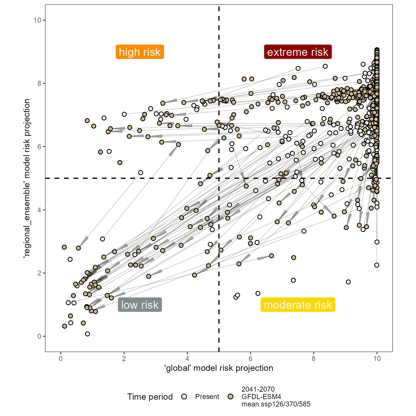

ggsave(
  xy_joined_rescaled_plot, 
  filename = file.path(
    here::here(), "vignette-outputs", "figures", "slf_risk_plot.jpg"
    ),
  height = 8, 
  width = 8,
  device = jpeg,
  dpi = "retina"
  )

# also save to rds
write_rds(
  xy_joined_rescaled_plot,
  file = file.path(here::here(), "vignette-outputs", "figures", "figures-rds", "slf_risk_plot.rds")
)

4. Create summary table of transformed plot

I will now create a summary table to explain the rescaled plots from step 4. The table will depict the quadrant placement of the point in the quadrant plot, both before and after climate change. From this, I will calculate the total number of movements into and out of each quadrant. I will apply the internal function scari::calculate_risk_quadrant().

I will create a summary table of the quadrant placement (and thus the level of risk) for each point in the IVR_locations dataset. I will use calculate_risk_quadrant() to accomplish this.

# create dataset and tidy
slf_populations_joined <- left_join(slf_populations, xy_joined_rescaled, by = c("x", "y")) %>%
  relocate(ID, x, y) 
  
# calculate risk quadrants
slf_populations_risk <- slf_populations_joined %>%
  mutate(
    risk_1995 = scari::calculate_risk_quadrant(
      suit.x = slf_populations_joined$xy_global_1995_rescaled,
      suit.y = slf_populations_joined$xy_regional_ensemble_1995_rescaled,
      thresh.x = global_MTSS, # this threshold remains the same
      thresh.y = regional_ensemble_MTSS_1995
    ),
    risk_2055 = scari::calculate_risk_quadrant(
      suit.x = slf_populations_joined$xy_global_2055_rescaled,
      suit.y = slf_populations_joined$xy_regional_ensemble_2055_rescaled,
      thresh.x = global_MTSS,
      thresh.y = regional_ensemble_MTSS_2055
    ),
    risk_shift = str_c(risk_1995, risk_2055, sep = "-")
  )

risk_levels <- c("extreme", "high", "moderate", "low")

slf_risk_table <- slf_populations_risk %>%
  # create counts and make into acrostic table
  dplyr::group_by(risk_1995, risk_2055) %>%
  dplyr::summarize(count = n()) %>%
  pivot_wider(names_from = risk_2055, values_from = count) %>%
  # tidy
  dplyr::rename("rows_1995_cols_2055" = "risk_1995") %>%
  relocate("rows_1995_cols_2055", "extreme", "high", "moderate") %>%
  arrange(factor(.$rows_1995_cols_2055, levels = risk_levels)) %>%
  # replace missing categories with 0
  replace(is.na(.), 0) %>%
  ungroup()

## `summarise()` has grouped output by 'risk_1995'. You can override using the
## `.groups` argument.

# tidy
slf_risk_table <- slf_risk_table %>%
  # add totals column
  tibble::add_column("total_present" = rowSums(.[, 2:5])) %>%
  # add row totals
  tibble::add_row(rows_1995_cols_2055 = "total_2055", extreme = colSums(dplyr::select(., 2)), high = colSums(dplyr::select(., 3)), moderate = colSums(dplyr::select(., 4)), low = colSums(dplyr::select(., 5)), total_present = 803)

write_csv(
  slf_risk_table, 
  file = file.path(here::here(), "vignette-outputs", "data-tables", "slf_risk_table.csv")
  )

5. global risk shift vs regional risk shift

I will create a table to sum the number of points in three different groups. My goal is to understand how the regional model adds resolution to our calculation of risk. So, I will look at how

I will sum the number of points that are suitable in the global model only, unsuitable in the global model only, and unsuitable in the global model / suitable in the regional model. I will repeat this operation for both time periods.

global_regional_risk_shift <- tibble(
  time_period = c(1995, 1995, 1995, 2055, 2055, 2055),
  quadrants = c("quad4_quad2", "quad3_quad1", "quad3", "quad4_quad2", "quad3_quad1", "quad3"),
  risk = c("extreme_moderate", "high_low", "high", "extreme_moderate", "high_low", "high"),
  model_suit = c("global_suit", "global_unsuit", "global_unsuit_regional_suit", "global_suit", "global_unsuit", "global_unsuit_regional_suit"),
  slf_population_count = c(
    # global suitable 1995
    sum(slf_populations_joined$xy_global_1995_rescaled >= global_MTSS),
    # global unsuitable 1995
    sum(slf_populations_joined$xy_global_1995_rescaled < global_MTSS),
    # global unsuitable and regional suitable 1995
    sum(slf_populations_joined$xy_global_1995_rescaled < global_MTSS & slf_populations_joined$xy_regional_ensemble_1995_rescaled >= regional_ensemble_MTSS_1995),
    # global suitable 2055
    sum(slf_populations_joined$xy_global_2055_rescaled >= global_MTSS),
    # global unsuitable 2055
    sum(slf_populations_joined$xy_global_2055_rescaled < global_MTSS),
    # global unsuitable and regional suitable 2055
    sum(slf_populations_joined$xy_global_2055_rescaled < global_MTSS & slf_populations_joined$xy_regional_ensemble_2055_rescaled >= regional_ensemble_MTSS_2055)
  )
)

# total # slf populations
total_slf <- sum(global_regional_risk_shift[1:2, 5])

global_regional_risk_shift <- mutate(
  global_regional_risk_shift, 
  slf_population_prop = slf_population_count / total_slf
  )


# calculate % of unsuit (quad3 and quad 1) that are are in quad3
quad3_risk_prop <- tibble(
  time_period = c("quad3_1995", "quad3_2055"),
  prop_total_unsuit_in_quad3 = c(
    scales::label_percent(accuracy = 0.01) (abs(as.numeric((global_regional_risk_shift[3, 5]) / global_regional_risk_shift[2, 5]))),
    scales::label_percent(accuracy = 0.01) (abs(as.numeric((global_regional_risk_shift[6, 5]) / global_regional_risk_shift[5, 5])))
  )
)

With this analysis, I found that currently, only about 2.9% of known (rarefied) SLF populations are low risk according to the global model. However, 1.1% of the total populations are specifically in quadrant 3 (high risk). This means that the global model alone would label 22 of the 769 slf populations as low risk, when in actuality 9 or about 40.9% of these are at high risk of persisting (above the MTSS threshold) when we spatially segment the presence data into an ensemble of regional-scale models. After climate change, 78 of the 1063 populations (10%) would be unsuitable if the global model alone were used to describe the risk of SLF. However, 22 or 28% of these unsuitable populations are still suitable in regional_scale models and thus would be missed by an analysis of risk using only a global-scale model.

This means that our regional-scale ensemble is adding resolution and nuance to our estimation of risk for SLF establishment.

# add %
global_regional_risk_shift <- mutate(global_regional_risk_shift, slf_population_prop = scales::label_percent(accuracy = 0.01) (slf_population_prop))

# make kable
global_regional_risk_shift <- kable(global_regional_risk_shift, "html", escape = FALSE) %>% 
  kableExtra::kable_styling(bootstrap_options = "striped", full_width = FALSE) %>%
  kableExtra::add_header_above(., header = c("SLF risk plot quadrant proportions" = 6), bold = TRUE)


# save as .html
kableExtra::save_kable(
  global_regional_risk_shift, 
  file = file.path(here::here(), "vignette-outputs", "figures", "slf_risk_plot_quadrant_props.html"),
  self_contained = TRUE
  )

# initialize webshot by 
# webshot::install_phantomjs()
# convert to pdf
webshot::webshot(
  url = file.path(here::here(), "vignette-outputs", "figures", "slf_risk_plot_quadrant_props.html"),
  file = file.path(here::here(), "vignette-outputs", "figures", "slf_risk_plot_quadrant_props.jpg"),
  zoom = 2
)


# rm html
file.remove(file.path(here::here(), "vignette-outputs", "figures", "slf_risk_plot_quadrant_props.html"))

References

Gallien, L., Douzet, R., Pratte, S., Zimmermann, N. E., & Thuiller, W. (2012). Invasive species distribution models – how violating the equilibrium assumption can create new insights. Global Ecology and Biogeography, 21(11), 1126–1136. https://doi.org/10.1111/j.1466-8238.2012.00768.x
Smith, T. 2021, August 11. Evaluating Invasion Stage with SDMs - plantarum.ca. https://plantarum.ca/2021/08/11/invasion-stage/.

Samuel M. Owens¹

2024-08-15

Overview

Setup

load rasters

tidy slf populations dataset

import and tidy xy suitability

take mean of global model ssp scenarios

retrieve suitability values for regional_ensemble

take mean of ssps

write to file

1. Transform xy suitability

2. Plot untransformed suitability values

3. plot transformed suitability values

find points that shift across thresholds

plot

4. Create summary table of transformed plot

5. global risk shift vs regional risk shift

References

Infer stability of known SLF populations due climate change effects

Samuel M. Owens1

2024-08-15

Overview

Setup

load rasters

tidy slf populations dataset

import and tidy xy suitability

take mean of global model ssp scenarios

retrieve suitability values for regional_ensemble

take mean of ssps

write to file

1. Transform xy suitability

2. Plot untransformed suitability values

3. plot transformed suitability values

find points that shift across thresholds

plot

4. Create summary table of transformed plot

5. global risk shift vs regional risk shift

References

Samuel M. Owens¹