Setup for global-scale MaxEnt model
Samuel M. Owens1
2025-07-07
Source:vignettes/040_setup_global_MaxEnt_model.Rmd
040_setup_global_MaxEnt_model.RmdOverview
In the previous vignette, I retrieved and formatted rasters of 19 global-scale climate variables from CHELSA. These represent some of the most relevant variables for the accomplishment of my goal, which is to explain the distribution for Lycorma delicatula according to climate. I also retrieved climate change versions of these variables, created by the CMIP6 climate modeling project. These variables were standardized and formatted for my needs. The most relevant variables were chosen for all future models.
The goal of this analysis is to train four models: a global model, a native range model, and two invaded models based on the invaded ranges in North America and east Asia. All three models will be based on historical (1981-2010) climate data and will be extrapolated for climate change using the CMIP6 rasters. Each model will be based on different training and testing ranges.
In this vignette, I will set up to run the global model and project it for climate change. I will need to format the data in this vignette, will be trained and tested on all available climate data that is split into 10 random folds. In the next vignette I will run this model, and in the following vignette I will set up for the three regional models.
| train_test_method | train_presences | test_presences | background_points |
|---|---|---|---|
| 10-fold random cross validation, 80% train / 20% test | 1026 | 256 | 20,000 |
Setup
I will prepare for this vignette by loading the necessary packages to run this script. I will also be creating maps during this analysis, so I will create a list object containing a standardized map style that I will continue to use.
library(tidyverse)  #data manipulation

library(here) #making directory pathways easier on different instances
# here() starts at the root folder of this package.

library(devtools)
library(dismo) # generate random background points

# spatial data handling
library(raster)
library(terra)

# aesthetics
library(webshot)
library(webshot2)
library(kableExtra)
library(patchwork)
Note: I will be setting the global options of this
document so that only certain code chunks are rendered in the final
.html file. I will set the eval = FALSE so that none of the
code is re-run (preventing files from being overwritten during knitting)
and will simply overwrite this in chunks with plots.
map_style <- list(
  theme_classic(),
  theme(
    legend.position = "bottom",
    panel.background = element_rect(fill = "lightblue2",colour = "lightblue2"),
    axis.title = element_blank(),
    axis.text = element_blank(),
    axis.ticks = element_blank()
    ),
  scale_x_continuous(expand = c(0, 0)),
  scale_y_continuous(expand = c(0, 0)),
  coord_equal()
)
1. Select Background Points for model
MaxEnt requires a set of “background” or “pseudoabsence” points that it will use to sample these rasters, which take the place of recorded absences. MaxEnt can randomly pick these internally, but it is more intuitive to manually select them. I can also account for latitudinal stretching of cell size and other factors if these are selected manually. Just for review, these points are used to characterize the variables that affect SLF distribution. Temperature / precipitation values will be extracted from the rasters for each point in this set. MaxEnt will then use these points to calculate an equation that describes the relationship of SLF with its environment and predict suitability. Note that only one set of background points need to be created for each of the global and regional models.
First, I will load in known SLF presences so that background sampling does not occur in those grid cells.
# dismo requires the base function (not tidyverse)
slf_points <- read_rds(file = file.path(here::here(), "data", "slf_all_coords_final_2025-07-07.rds")) %>%
  dplyr::select(-species) %>%
  as.data.frame()
# file path to local directory
mypath <- file.path(here::here() %>%
                     dirname(),
                   "maxent/historical_climate_rasters/chelsa2.1_30arcsec/v1_maxent_10km")
Gallien et.al recommended 20,000 points for background with a
global-scale model. Gallien also found that a higher number of
background points artificially deflates MaxEnt predicitons, so it is
important not to choose too many. However, it is appropriate to scale
the datasets according to the spatial scale of the rasters. Initially, I
selected 42,523 random background points using
dismo::randomPoints(), because Santana Jr et.al recommended
this amount when modeling at a global scale (Santana Jr et.al, 2019).
These models were incredibly specific and overfit, and the models were
incredible complex, so I downgraded the point count to 20,000.
Note that I will be running this analysis at the 10km scale, so I
need to use the 10km rasters to ensure that points are chosen with
appropriate spacing. These datasets will be stored in
vignette-outputs/data-tables.
# load in reference layer. needs to be done with raster package because dismo doesnt recognize terra package objects
global_bio2 <- raster::raster(x = file.path(mypath, "bio2_1981-2010_global.asc"))
# check number of cells
terra::ncell(global_bio2)
# check crs
terra::crs(global_bio2)
# plenty of cells to work with if we remove those with SLF points

# set seed so that the random points for this dataset are the same the next time this code is run
set.seed(1.5)
# generate random points
global_points <- dismo::randomPoints(
  mask = global_bio2,
  n = 20000, # double the default number used by maxent
  p = slf_points,
  excludep = TRUE, # exclude cells where slf has been found
  lonlatCorrection = FALSE, # was previously true but not necessary in ESRI 54017
  warn = 2 # higher number gives most warnings, including if sample size not reached
  ) %>%
  as.data.frame(.)

# save as csv
write_csv(x = global_points, file = file.path(here::here(), "vignette-outputs", "data-tables", "global_background_points_v4.csv"))
# save as rds file
write_rds(global_points, file = file.path(here::here(), "data", "global_background_points_v4.rds"))
Now, I will plot these points for visualization purposes.
mypath <- file.path(here::here() %>%
                     dirname(),
                   "maxent/historical_climate_rasters/chelsa2.1_30arcsec/v1_maxent_10km")

# background layer
global_bio2_df <- terra::rast(x = file.path(mypath, "bio2_1981-2010_global.asc")) %>%
  terra::as.data.frame(., xy = TRUE)
# points
global_points <- read_csv(file = file.path(here::here(), "vignette-outputs", "data-tables", "global_background_points_v4.csv"))
## Warning: Raster pixels are placed at uneven horizontal intervals and will be shifted
## ℹ Consider using `geom_tile()` instead.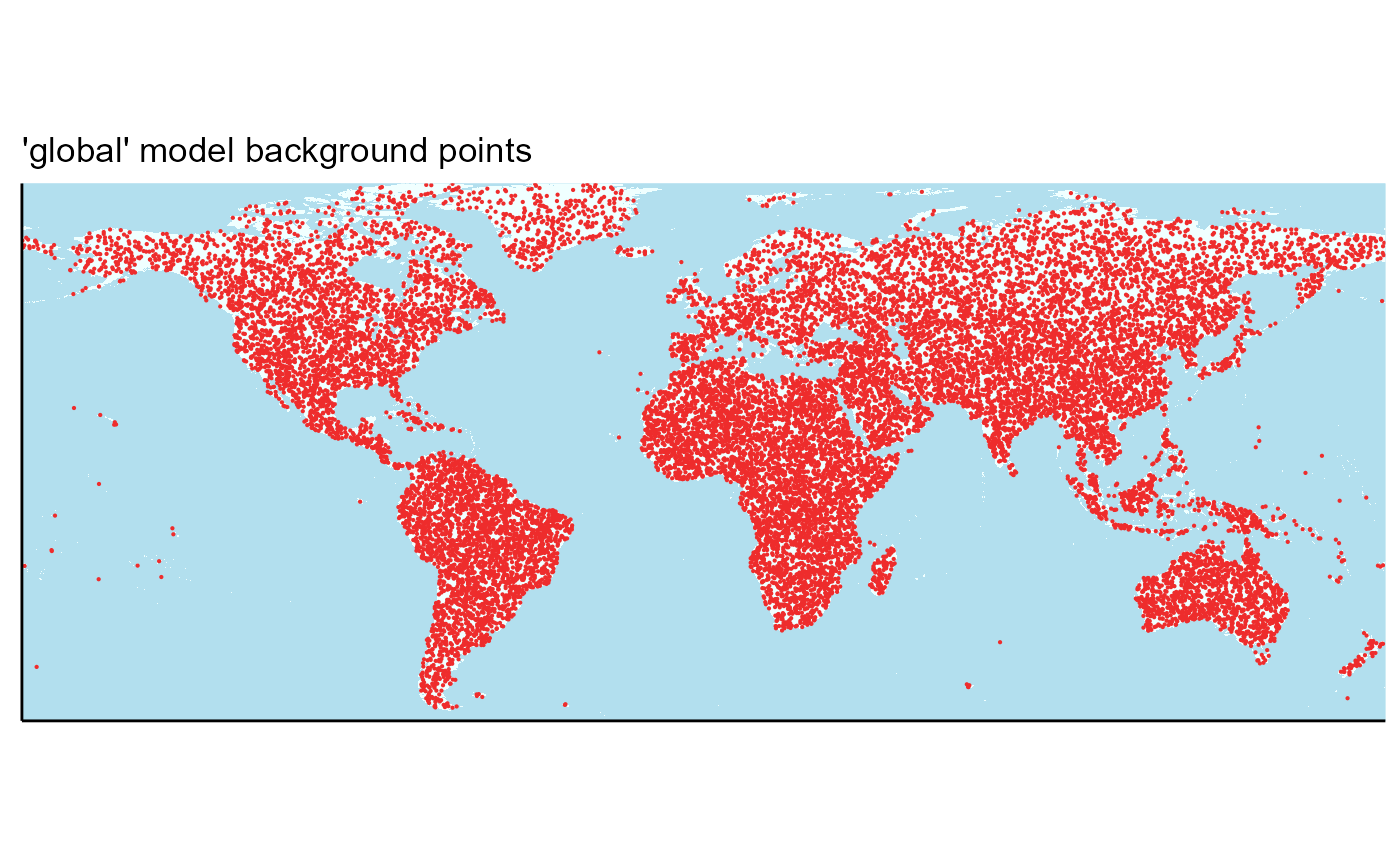
2. Plot SLF presences
Now I will create a plot of all SLF presence locations for reference. These points will represent the known presences in the model.
## Warning: Raster pixels are placed at uneven horizontal intervals and will be shifted
## ℹ Consider using `geom_tile()` instead.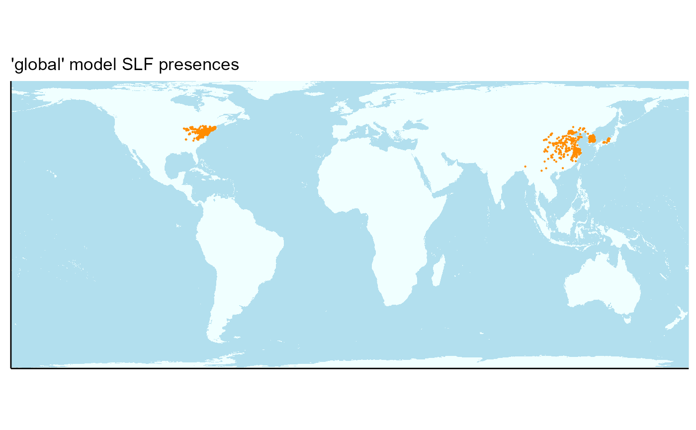
ggsave(
  global_slf_plot,
  filename = file.path(here::here(), "vignette-outputs", "figures", "global_model_presence_points_v4.jpg"),
  height = 8,
  width = 12,
  device = jpeg,
  dpi = 500
  )
Now that we have selected the background point datasets and created rasters for training and projection purposes, we are ready to run our models. The next vignette will train and project the global model, while the following vignette will perform a similar setup for the regional model.
References
Calvin, D. D., Rost, J., Keller, J., Crawford, S., Walsh, B., Bosold, M., & Urban, J. (2023). Seasonal activity of spotted lanternfly (Hemiptera: Fulgoridae), in Southeast Pennsylvania. Environmental Entomology, 52(6), 1108–1125. https://doi.org/10.1093/ee/nvad093
Gallien, L., Douzet, R., Pratte, S., Zimmermann, N. E., & Thuiller, W. (2012). Invasive species distribution models – how violating the equilibrium assumption can create new insights. Global Ecology and Biogeography, 21(11), 1126–1136. https://doi.org/10.1111/j.1466-8238.2012.00768.x
Santana Jr, P. A., Kumar, L., Da Silva, R. S., Pereira, J. L., & Picanço, M. C. (2019). Assessing the impact of climate change on the worldwide distribution of Dalbulus maidis (DeLong) using MaxEnt. Pest Management Science, 75(10), 2706–2715. https://doi.org/10.1002/ps.5379