Check model goodness of fit via AUC, TSS and confusion matrices
Samuel M. Owens1
2024-08-16
Source:vignettes/141_plot_AUC_var_cont.Rmd
141_plot_AUC_var_cont.RmdI will plot the AUC curves and variable contribution graphs by combining all 4 models into one plot. This will allow for a direct comparison of the AUC (goodness of fit) and var contribution between models.
Setup
# general tools
library(tidyverse)  #data manipulation
library(here) #making directory pathways easier on different instances
# here::here() starts at the root folder of this package.
library(devtools)

# SDMtune and dependencies
library(SDMtune) # main package used to run SDMs
library(dismo) # package underneath SDMtune
library(rJava) # for running MaxEnt
library(plotROC) # plots ROCs

# html tools
library(kableExtra)
library(webshot)
library(webshot2)
These plots depict the activity of the variables put into the MaxEnt models. I will create a combined figure for the 3 models in the regional_ensemble
ensemble_colors <- c(
  "Rn (native)" = "#4daf4a",
  "Ri.NAmerica" =  "#e41a1c",
  "Ri.Asia" = "#377eb8"
)
regional_native_model <- read_rds(file = file.path(mypath, "slf_regional_native_v3", "regional_native_model.rds"))

regional_invaded_model <- read_rds(file = file.path(mypath, "slf_regional_invaded_v7", "regional_invaded_model.rds"))

regional_invaded_asian_model <- read_rds(file = file.path(mypath, "slf_regional_invaded_asian_v2", "regional_invaded_asian_model.rds"))
regional_native_test <- read_rds(file = file.path(mypath, "slf_regional_native_v3", "regional_native_test.rds"))

regional_invaded_test <- read_rds(file = file.path(mypath, "slf_regional_invaded_v7", "regional_invaded_test.rds"))

regional_invaded_asian_test <- read_rds(file = file.path(mypath, "slf_regional_invaded_asian_v2", "regional_invaded_asian_test.rds"))
ROC regional ensemble
regional_native_ROC <- SDMtune::plotROC(
  model = regional_native_model,
  test = regional_native_test
) %>%
  ggplot_build()


regional_invaded_ROC <- SDMtune::plotROC(
  model = regional_invaded_model,
  test = regional_invaded_test
) %>%
  ggplot_build()

regional_invaded_asian_ROC <- SDMtune::plotROC(
  model = regional_invaded_asian_model,
  test = regional_invaded_asian_test
) %>%
  ggplot_build()
ROC_ensemble <- ggplot() +
  # native model data
  geom_line(data = regional_native_ROC$data[[1]], aes(x = x, y = y, color = "Rn (native)", group = group, linetype = as.factor(group)), linewidth = 0.8) +
  # invaded model data
  geom_line(data = regional_invaded_ROC$data[[1]], aes(x = x, y = y, color = "Ri.NAmerica", group = group, linetype = as.factor(group)), linewidth = 0.8) +
  # invaded_asian model data
  geom_line(data = regional_invaded_asian_ROC$data[[1]], aes(x = x, y = y, color = "Ri.Asia", group = group, linetype = as.factor(group)), linewidth = 0.8) +
  # midpoint line
  geom_abline(slope = 1, linetype = "dashed") +
  # scales
  scale_x_continuous(name = "False positive rate (1 - specificity)", breaks = c(0, 0.25, 0.5, 0.75, 1), limits = c(0, 1)) +
  scale_y_continuous(name = "True positive rate (sensitivity)", breaks = c(0, 0.25, 0.5, 0.75, 1), limits = c(0, 1)) +
  labs(
    title = "ROC curve (true vs false positive rate) for 'regional_ensemble' models"
    ) +
  theme_bw() +
  # aes
  scale_color_manual(
    name = "model",
    values = ensemble_colors,
    aesthetics = "color"
  ) +
  scale_linetype_manual(
    name = "Data segment",
    values = c("solid", "dotted"),
    labels = c("Test", "Train"),
    guide = guide_legend(reverse = TRUE)
  ) +
  theme(legend.position = "bottom") +
coord_fixed(ratio = 1)Add global model to AUC plot
ROC
global_model <- read_rds(file = file.path(mypath, "slf_global_v3", "global_model.rds"))
global_test <- read_rds(file = file.path(mypath, "slf_global_v3", "global_test.rds"))

ensemble_colors <- c(
  "Rn (native)" = "#4daf4a",
  "Ri.NAmerica" =  "#e41a1c",
  "Ri.Asia" = "#377eb8",
  "global" = "black"
)
global_ROC <- SDMtune::plotROC(
  model = global_model@models[[5]], #pick one because they did not vary too much
  test = global_test
) %>%
  ggplot_build()
ROC_ensemble_global <- ggplot() +
  # global
  geom_line(data = global_ROC$data[[1]], aes(x = x, y = y, color = "global", group = group, linetype = as.factor(group)), linewidth = 0.8) +
  # native model data
  geom_line(data = regional_native_ROC$data[[1]], aes(x = x, y = y, color = "Rn (native)", group = group, linetype = as.factor(group)), linewidth = 0.8) +
  # invaded model data
  geom_line(data = regional_invaded_ROC$data[[1]], aes(x = x, y = y, color = "Ri.NAmerica", group = group, linetype = as.factor(group)), linewidth = 0.8) +
  # invaded_asian model data
  geom_line(data = regional_invaded_asian_ROC$data[[1]], aes(x = x, y = y, color = "Ri.Asia", group = group, linetype = as.factor(group)), linewidth = 0.8) +
  # midpoint line
  geom_abline(slope = 1, linetype = "dashed") +
  # scales
  scale_x_continuous(name = "False positive rate (1 - specificity)", breaks = c(0, 0.25, 0.5, 0.75, 1), limits = c(0, 1)) +
  scale_y_continuous(name = "True positive rate (sensitivity)", breaks = c(0, 0.25, 0.5, 0.75, 1), limits = c(0, 1)) +
  labs(
    title = "ROC curve (true vs false positive rate) for 'regional_ensemble' and 'global' models"
    ) +
  theme_bw() +
  # aes
  scale_color_manual(
    name = "model",
    values = ensemble_colors,
    aesthetics = "color"
  ) +
  scale_linetype_manual(
    name = "Data segment",
    values = c("solid", "dotted"),
    labels = c("Test", "Train"),
    guide = guide_legend(reverse = TRUE)
  ) +
  theme(legend.position = "bottom") +
  coord_fixed(ratio = 1)

ROC_ensemble_global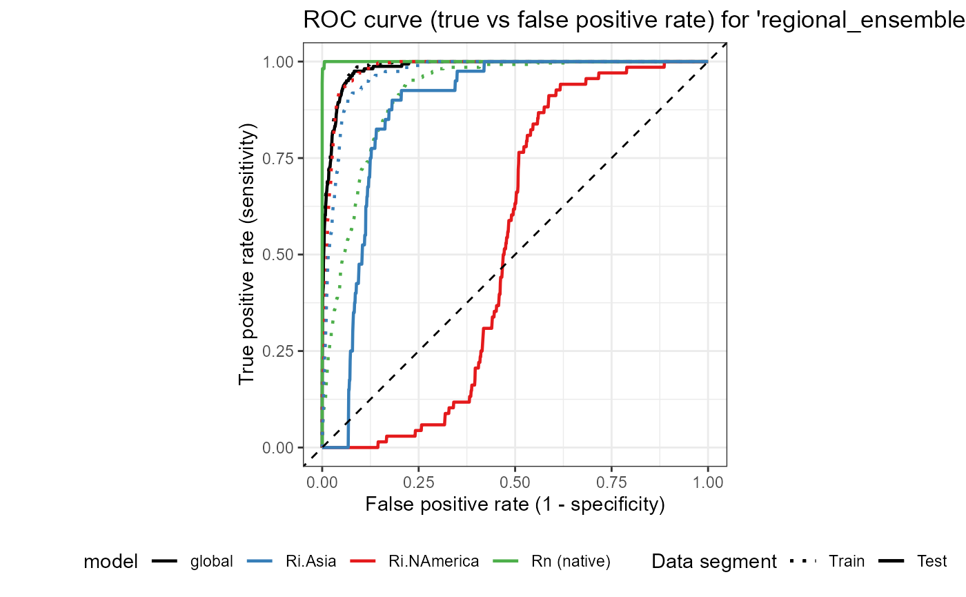
ggsave(
  ROC_ensemble_global,
  filename = file.path(
    here::here(), "vignette-outputs", "figures", "ROC_plot_regional_ensemble_global.jpg"
    ),
  height = 8,
  width = 8,
  device = jpeg,
  dpi = "retina"
  )
I will create a table for some important summary statistics for the models. These include sensitivity, specificity, commission error, and omission error. These are calculated according to the cloglog MTSS threshold per model.
Sensitivity and Specificity of Models
We calculate these according to the cloglog MTSS threshold per model
# global
global_conf_matr <- read_csv(file = file.path(mypath, "slf_global_v3", "global_thresh_confusion_matrix_all_iterations.csv")) %>%
  # only MTSS threshold
  slice(7)
## Rows: 9 Columns: 6
## ── Column specification ────────────────────────────────────────────────────────
## Delimiter: ","
## chr (1): threshold_type
## dbl (5): threshold_value, tp_mean, fp_mean, fn_mean, tn_mean
##
## ℹ Use `spec()` to retrieve the full column specification for this data.
## ℹ Specify the column types or set `show_col_types = FALSE` to quiet this message.
# regional models
# native
regional_native_conf_matr <- read_csv(file = file.path(mypath, "slf_regional_native_v3", "regional_native_thresh_confusion_matrix.csv")) %>%
  slice(7)
## Rows: 9 Columns: 6
## ── Column specification ────────────────────────────────────────────────────────
## Delimiter: ","
## chr (1): threshold_type
## dbl (5): threshold_value, tp, fp, fn, tn
##
## ℹ Use `spec()` to retrieve the full column specification for this data.
## ℹ Specify the column types or set `show_col_types = FALSE` to quiet this message.
# invaded_asia
regional_invaded_asian_conf_matr <- read_csv(file = file.path(mypath, "slf_regional_invaded_asian_v2", "regional_invaded_asian_thresh_confusion_matrix.csv")) %>%
  slice(7)
## Rows: 9 Columns: 6
## ── Column specification ────────────────────────────────────────────────────────
## Delimiter: ","
## chr (1): threshold_type
## dbl (5): threshold_value, tp, fp, fn, tn
##
## ℹ Use `spec()` to retrieve the full column specification for this data.
## ℹ Specify the column types or set `show_col_types = FALSE` to quiet this message.
# invaded_NAmerica
regional_invaded_conf_matr <- read_csv(file = file.path(mypath, "slf_regional_invaded_v7", "regional_invaded_thresh_confusion_matrix.csv")) %>%
  slice(7)
## Rows: 9 Columns: 6
## ── Column specification ────────────────────────────────────────────────────────
## Delimiter: ","
## chr (1): threshold_type
## dbl (5): threshold_value, tp, fp, fn, tn
##
## ℹ Use `spec()` to retrieve the full column specification for this data.
## ℹ Specify the column types or set `show_col_types = FALSE` to quiet this message.Be sure to change the number of test positives and background negatives for each model if this changes.
model_sens_spec <- tibble(
  metric = rep(c("sensitivity", "specificity", "commission error", "omission error"), 4),
  description = rep(c("true_positive rate", "true_negative rate", "1 - true_negative rate", "false_negative rate"), 4),
    model = c(
    rep("global", 4),
    rep("regional\nnative", 4),
    rep("regional\ninvaded NAmerica", 4),
    rep("regional\ninvaded Asia", 4)
  ),
  thresh = "MTSS.cloglog",
  thresh_value = c(
    rep(global_conf_matr$threshold_value, 4),
    rep(regional_native_conf_matr$threshold_value, 4),
    rep(regional_invaded_conf_matr$threshold_value, 4),
    rep(regional_invaded_asian_conf_matr$threshold_value, 4)
    ),
  test_pos = c(
    rep(155, 4), # global
    rep(54, 4),  # native
    rep(68, 4), # invaded_NAmerica
    rep(40, 4) # invaded_Asia
  ),
  bg_neg = c(
    rep(20000, 4), # global
    rep(10000, 12) # regional
  ),
  value = c(
    # global
    round(global_conf_matr$tp_mean / 155, 4), round(global_conf_matr$tn_mean / 20000, 4), round(1 - (global_conf_matr$tn_mean / 20000), 4), round((global_conf_matr$fn_mean / 20000), 4),
    # native
    round(regional_native_conf_matr$tp / 54, 4), round(regional_native_conf_matr$tn / 10000, 4), round(1 - (regional_native_conf_matr$tn / 10000), 4), round((regional_native_conf_matr$fn / 10000), 4),
    # invaded_NAmerica
    round(regional_invaded_conf_matr$tp / 68, 4), round(regional_invaded_conf_matr$tn / 10000, 4), round(1 - (regional_invaded_conf_matr$tn / 10000), 4), round((regional_invaded_conf_matr$fn / 10000), 4),
    # invaded_asia
    round(regional_invaded_asian_conf_matr$tp / 40, 4), round(regional_invaded_asian_conf_matr$tn / 10000, 4), round(1 - (regional_invaded_asian_conf_matr$tn / 10000), 4), round((regional_invaded_asian_conf_matr$fn / 10000), 4)
  )
)
write_csv(model_sens_spec, file.path(here::here(), "vignette-outputs", "data-tables", "model_sensitivity_specificity.csv"))I will also write it to a kable so it can be printed
# add column formatting
model_sens_spec <- mutate(model_sens_spec, bg_neg = scales::label_comma() (bg_neg))

# convert to kable
model_sens_spec_kable <- knitr::kable(x = model_sens_spec, format = "html", escape = FALSE) %>%
  kableExtra::kable_styling(bootstrap_options = "striped", full_width = TRUE)

# save as .html
kableExtra::save_kable(
  model_sens_spec_kable,
  file = file.path(here::here(), "vignette-outputs", "figures", "model_sensitivity_specificity.html"),
  self_contained = TRUE,
  bs_theme = "simplex"
  )

# initialize webshot by
# webshot::install_phantomjs()
# convert to pdf
webshot::webshot(
  url = file.path(here::here(), "vignette-outputs", "figures", "model_sensitivity_specificity.html"),
  file = file.path(here::here(), "vignette-outputs", "figures", "model_sensitivity_specificity.jpg"),
  zoom = 2
)

# model extents

model_sens_spec_kable
References
Jiménez‐Valverde, A. (2012). Insights into the area under the receiver operating characteristic curve (AUC) as a discrimination measure in species distribution modelling. Global Ecology and Biogeography, 21(4), 498–507. https://doi.org/10.1111/j.1466-8238.2011.00683.x
Zou, K. H., O’Malley, A. J., & Mauri, L. (2007). Receiver-Operating Characteristic Analysis for Evaluating Diagnostic Tests and Predictive Models. Circulation, 115(5), 654–657. https://doi.org/10.1161/CIRCULATIONAHA.105.594929