Plot shift in SLF risk to important viticultural regions under climate change

Overview

In the last vignette, I created risk maps and range shift maps as the first step in visualizing and comparing the predictions made by my global and regional ensemble models. I will apply these maps for drawing on general trends of SLF suitable area shift under climate change. Downstream, I also plan to visualize these suitability maps across geographical regions and at a finer scale, such as for viticulturally important countries and provinces.

In this vignette, I will focus on making more specific predictions for SLF establishment risk scatter plots of the suitability values for the globally important viticultural regions in the global and regional ensemble models. I will use a quadrant scatter plot to visualize the movement of these regions across the minimum threshold suitability value (the MTSS value). By plotting one model scale on each axis, we can visualize the agreement between our modeled scales.

Gallien et al, 2012 originally defined this method for discerning the “stage of invasion” for invasive populations according to different scales of SDM. I will apply this method and re-interpret it as a method for assessing the risk of establishment. These two models will not completely agree on the suitability for a particular location, so agreement between the modeled scales can give us more confidence in that prediction. Where the modeled scales disagree, we might make different interpretations of the biological mechanism at play.

## ── Attaching core tidyverse packages ──────────────────────── tidyverse 2.0.0 ──
## ✔ dplyr     1.1.4     ✔ readr     2.1.5
## ✔ forcats   1.0.0     ✔ stringr   1.5.1
## ✔ ggplot2   3.5.2     ✔ tibble    3.3.0
## ✔ lubridate 1.9.4     ✔ tidyr     1.3.1
## ✔ purrr     1.0.4     
## ── Conflicts ────────────────────────────────────────── tidyverse_conflicts() ──
## ✖ dplyr::filter() masks stats::filter()
## ✖ dplyr::lag()    masks stats::lag()
## ℹ Use the conflicted package (<http://conflicted.r-lib.org/>) to force all conflicts to become errors

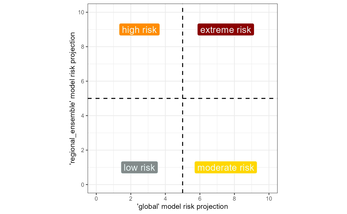Fig. 1 Example quadrant plot for assessing SLF risk across two different scales of SDM.

We rate risk from low to extreme, based on the agreement between the modeled scales. We rate suitability in the regional_ensemble only (top left, high) as higher risk than suitability in the global model only (bottom right, moderate) because we believe that unique suitability in the regional-scale ensemble indicates a risk for adaptation to new climatic niches (Gallien et al, 2012). Where the regional-scale model detects suitability when the global model cannot, SLF might be adapting to a climatic niche outside its global mean niche.

The MTSS threshold of suitability will be used as the central crosshairs of this plot. We will then plot the same set of points presently and in the future under our climate change scenarios. Movement across the MTSS threshold on either axis due to climate change will indicate that climate change is changing the suitability of these regions for SLF establishment. I will need to transform these suitability values so that the MTSS threshold falls on 0.5. This will allow me to visualize the movement of these regions across the minimum threshold suitability value.

First, I will plot the un-transformed version of the data and then will transform and plot the data again. I will use a table to calculate the number of regions that move across the MTSS threshold and fall into each category before and after climate change. Finally, I will save the predicted suitability values with our wineries dataset for downstream analysis. Our wineries.rda dataset contains the locations of 1,086 globally important viticultural regions.

Setup

# general tools
library(tidyverse)  #data manipulation
library(here) #making directory pathways easier on different instances
# here() starts at the root folder of this package.
library(devtools)

# spatial data handling
library(terra)
library(CoordinateCleaner)

# plot aesthetics
library(scales)
library(patchwork)
library(grid)
library(kableExtra)
library(webshot)
library(webshot2)

# this package
library(scari)

Note: I will be setting the global options of this document so that only certain code chunks are rendered in the final .html file. I will set the eval = FALSE so that none of the code is re-run (preventing files from being overwritten during knitting) and will simply overwrite this in chunks with plots.

mypath <- file.path(here::here() %>% 
                       dirname(),
                     "maxent/models")

I will load in some aesthetic objects for plotting.

breaks <- c(0.0, 0.2, 0.4, 0.6, 0.8, 1.0)

labels <- c(0, 2, 4, 6, 8, 10)

load rasters

Load in summary files for the global and regional ensemble models, which contain the thresholds.

# summary file to extract thresholds from

# global
summary_global <- read_csv(file = file.path(mypath, "slf_global_v4", "global_summary_all_iterations.csv"))

summary_regional_ensemble <- read_csv(file = file.path(mypath, "slf_regional_ensemble_v2", "ensemble_threshold_values.csv"))

I will load in the global and regional ensemble suitability maps. These will be used both for extracting the new xy suitability values and for plotting.

# global
global_1995 <- terra::rast(x = file.path(mypath, "slf_global_v4", "global_pred_suit_clamped_cloglog_globe_1981-2010_mean.asc"))

global_2055 <- terra::rast(x = file.path(mypath, "slf_global_v4", "global_pred_suit_clamped_cloglog_globe_2041-2070_GFDL_ssp_averaged.asc"))


# regional_ensemble
# historical
regional_ensemble_1995 <- terra::rast(
  x = file.path(mypath, "slf_regional_ensemble_v2", "ensemble_regional_weighted_mean_globe_1981-2010.asc")
  )
# CMIP6
## ssp 126
regional_ensemble_2055_126 <- terra::rast(
  x = file.path(mypath, "slf_regional_ensemble_v2", "ensemble_regional_weighted_mean_globe_2041-2070_GFDL_ssp126.asc")
  )
# ssp 370
regional_ensemble_2055_370 <- terra::rast(
  x = file.path(mypath, "slf_regional_ensemble_v2", "ensemble_regional_weighted_mean_globe_2041-2070_GFDL_ssp370.asc")
  )
# ssp 585
regional_ensemble_2055_585 <- terra::rast(
  x = file.path(mypath, "slf_regional_ensemble_v2", "ensemble_regional_weighted_mean_globe_2041-2070_GFDL_ssp585.asc")
  )
# ssp mean
regional_ensemble_2055_ssp_mean <- terra::rast(
  x = file.path(mypath, "slf_regional_ensemble_v2", "ensemble_regional_weighted_mean_globe_2041-2070_GFDL_ssp_averaged.asc")
  )

tidy wineries dataset

I will load in dataset containing locations of globally important viticultural regions. I will also de-duplicate the records because there were “many-to-many” joining matches downstream. De-duplicating removed about 17 records. I also remove the species column, which is automatically created by SDMtune::predict() upstream.

# load in OG (not transformed) wineries dataset- transformed is wineries_esri54017.rds
# coordinatecleaner requires latlon
load(file.path(here::here(), "data-raw", "wineries.rda"))

IVR_locations <- wineries %>%
  # tidy
  dplyr::select(-c(Latitude, Longitude)) %>%
  dplyr::filter(
    !is.na(x),
    !is.na(y)
    ) %>%
  dplyr::mutate(record_type = "IVR_location")

# remove duplicate coordinates
IVR_locations <- CoordinateCleaner::clean_coordinates(
  x = IVR_locations,
  lon = "x",
  lat = "y",
  species = "record_type",
  tests = "duplicates",
  value = "clean" # just return same df without duplicates
) %>%
  dplyr::select(-record_type)

# remove unnecessary obj
rm(wineries)

import and tidy xy suitability

These scatter plots will be based on the suitability for the IVR points in both the global and regional_ensemble models. I have already calculated the xy suitability for the global model based on these points, using the function scari::predict_xy_suitability(). This function will not work for the regional_ensemble because it calls for a model object, which we did not use to predict the ensemble suitability. So, I will use terra::extract() to perform this action.

I will load in the global model datasets and create the regional_ensemble datasets. I will also do some tidying of my datasets for the plots I will create.

# historical
xy_global_1995 <- read_csv(
  file = file.path(mypath, "slf_global_v4", "global_wineries_1981-2010_xy_pred_suit_clamped_cloglog_mean_20000m_buffer.csv")
  ) 

# CMIP6
## ssp 126
xy_global_2055_126 <- read_csv(
  file = file.path(mypath, "slf_global_v4", "global_wineries_2041-2070_GFDL_ssp126_xy_pred_suit_clamped_cloglog_mean_20000m_buffer.csv")
  ) 
## ssp 370
xy_global_2055_370 <- read_csv(
  file = file.path(mypath, "slf_global_v4", "global_wineries_2041-2070_GFDL_ssp370_xy_pred_suit_clamped_cloglog_mean_20000m_buffer.csv")
  ) 
## ssp 585
xy_global_2055_585 <- read_csv(
  file = file.path(mypath, "slf_global_v4", "global_wineries_2041-2070_GFDL_ssp585_xy_pred_suit_clamped_cloglog_mean_20000m_buffer.csv")
  )

I need to add something I am calling a “join_col”. These columns are simply the main coordinate data, but rounded to a higher decimal place. This is to account for a CRS in meters UTM, which involves a very specific number. When I join the datasets downstream, they will not join correctly downstream without rounding.

Additionally, I need to rename each coordinate column to reflect its column of origin. This way, I will not lose track of which column is from which data frame among a veritable mess of joins.

# add join columns to all datasets
xy_global_1995 <- xy_global_1995 %>%
    dplyr::mutate(
      join_col_x = round(x, 5),
      join_col_y = round(y, 4) # rounding to the 1000s (1km) place to prevent overly sensitive exclusions for UTM data
    ) %>%
  # rename original cols to keep straight during joins
  dplyr::rename(
    x_global_1995 = x,
    y_global_1995 = y
  ) 

xy_global_2055_126 <- xy_global_2055_126 %>%
    dplyr::mutate(
      join_col_x = round(x, 5),
      join_col_y = round(y, 4) # rounding to the 1000s (1km) place to prevent overly sensitive exclusions for UTM data
    ) %>%
   dplyr::rename(
      x_global_2055_126 = x,
      y_global_2055_126 = y,
      "max_cloglog_suit_ssp126" = "max_cloglog_suitability_20000m_buffer" # rename max column for joining later
    ) 


xy_global_2055_370 <- xy_global_2055_370 %>%
    dplyr::mutate(
      join_col_x = round(x, 5),
      join_col_y = round(y, 4) # rounding to the 1000s (1km) place to prevent overly sensitive exclusions for UTM data
    ) %>%
   dplyr::rename(
      x_global_2055_370 = x,
      y_global_2055_370 = y,
      "max_cloglog_suit_ssp370" = "max_cloglog_suitability_20000m_buffer"
    ) 

xy_global_2055_585 <- xy_global_2055_585 %>%
    dplyr::mutate(
      join_col_x = round(x, 5),
      join_col_y = round(y, 4) # rounding to the 1000s (1km) place to prevent overly sensitive exclusions for UTM data
    ) %>%
   dplyr::rename(
      x_global_2055_585 = x,
      y_global_2055_585 = y,
      "max_cloglog_suit_ssp585" = "max_cloglog_suitability_20000m_buffer"
    )

I will need to create versions that are transformed to the the EPSG4326 CRS because coordinate cleaner does not work with ESRI:54017. I will also de-duplicate these datasets to ensure that there are no duplicate coordinates, which would cause problems with the terra::extract() function.

# 1995 historical dataset
# I need to transform this dataset to the correct crs
xy_global_1995_sv <- terra::vect(xy_global_1995, geom = c("x_global_1995", "y_global_1995"), crs = "ESRI:54017") %>%
    terra::project(y = "EPSG:4326") %>% # convert to UTM 33N
# convert to geom, which gets coordinates of a spatVector
    terra::geom()
# convert back to data frame
xy_global_1995_epsg4326 <- terra::as.data.frame(xy_global_1995_sv) %>%
    dplyr::select(-c(geom, part, hole)) %>%
    dplyr::rename("x_latlon" = "x", "y_latlon" = "y") 

# bind OG data
xy_global_1995_epsg4326 <- cbind(xy_global_1995_epsg4326, xy_global_1995) %>% 
  dplyr::select(-c(x_global_1995, y_global_1995)) 

rm(xy_global_1995_sv)



# de-duplicate just to make sure
xy_global_1995_epsg4326 <- xy_global_1995_epsg4326 %>%
  dplyr::mutate(species = "Lycorma delicatula") %>%
  CoordinateCleaner::clean_coordinates(
    x = .,
    lon = "x_latlon",
    lat = "y_latlon",
    species = "species",
    tests = "duplicates",
    value = "clean"
  ) 

rm(xy_global_1995_epsg4326)

The coordinates are the same across the other datasets (126, 370, 585), so we can assume they are all deduplicated.

The xy_suitabilities for the global models also contain a few less records than the IVR regions. To ensure that I am retrieving the suitability values for the exact same vineyards in the regional_ensemble, I will perform a filtering join. The IVR dataset should now contain the same records as the global suitability values do.

First, I need to transform the coordinates to the ESRI:54017 CRS

# I need to transform this dataset to the correct crs
IVR_locations_sv <- terra::vect(IVR_locations, geom = c("x", "y"), crs = "EPSG:4326") %>%
    terra::project(y = "ESRI:54017") %>% # convert to UTM 33N
# convert to geom, which gets coordinates of a spatVector
    terra::geom()
# convert back to data frame
IVR_locations_UTM <- terra::as.data.frame(IVR_locations_sv) %>%
    dplyr::select(-c(geom, part, hole)) %>%
    dplyr::rename("x_utm" = "x", "y_utm" = "y") 

# bind OG data
IVR_locations_UTM <- cbind(IVR_locations_UTM, IVR_locations) %>% 
  dplyr::select(-c(x, y)) %>% 
  dplyr::rename("x" = "x_utm", "y" = "y_utm")

Now, perform a filtering join and save

# edits to IVR dataset for rounding- create a join column
IVR_locations_join <- IVR_locations_UTM %>%
    dplyr::mutate(
      join_col_x = round(x, 5),
      join_col_y = round(y, 4) # rounding to the 1000s (1km) place to prevent overly sensitive exclusions for UTM data
    )
# join col already in xy_global_1995

# join with filtering join to keep least number of common records
IVR_locations_join <-  semi_join(IVR_locations_join, xy_global_1995, by = c("join_col_x", "join_col_y")) 
# this join worked, kept 1,072 records

# add ID column
IVR_locations_join <- IVR_locations_join %>%
  # create ID col
  dplyr::mutate(ID = row_number()) %>%
  # remove join columns
  dplyr::select(-c(join_col_x, join_col_y)) %>%
  relocate(ID, x, y) 

# save transformation for future use
readr::write_rds(x = IVR_locations_join, file = file.path(here::here(), "data", "wineries_esri54017_tidied.rds"))

# remove
rm(IVR_locations)
rm(IVR_locations_sv)
rm(IVR_locations_UTM)
rm(IVR_locations_join)

#read it back in
IVR_locations <- readr::read_rds(file.path(here::here(), "data", "wineries_esri54017_tidied.rds"))

take mean of global model ssp scenarios

I will take the mean of the suitability value within each of these predicted suitability datasets. These suitability values were taken from a 20km buffer around each viticultural area point to account for the potentially large size of these viticultural areas. We will keep the max values from those buffers. I will mean these values across ssp scenarios.

# first join datasets
xy_global_2055_ssp_mean <- xy_global_2055_126 %>%
  dplyr::left_join(., xy_global_2055_370, by = c("join_col_x", "join_col_y")) %>%
  dplyr::left_join(., xy_global_2055_585, by = c("join_col_x", "join_col_y")) %>%
  dplyr::relocate(max_cloglog_suit_ssp126, max_cloglog_suit_ssp370, max_cloglog_suit_ssp585) %>%
  # take mean of columns
  dplyr::mutate(max_suit_ssp_averaged = rowMeans(.[, 1:3])) %>%
  dplyr::select(x_global_2055_126, y_global_2055_126, max_suit_ssp_averaged) %>%
  # rename for saving
  dplyr::rename(
    x = x_global_2055_126,
    y = y_global_2055_126
  )

write_csv(
  x = xy_global_2055_ssp_mean,
  file = file.path(mypath, "slf_global_v4", "global_wineries_2041-2070_GFDL_ssp_mean_xy_pred_suit_clamped_cloglog_mean_20000m_buffer.csv")
    )

retrieve suitability values for regional_ensemble

Now, I will retrieve the suitability values for the regional_ensemble using the 20km buffer method described above. I will use buffer() and zonal() from the terra package to first create these 20km buffers around each point, then to take zonal statistics (the max value) from each buffer zone.

Instead of returning the coordinates from the map, I will join the coordinates from the original IVR_locations dataset so that the coordinates are exact for joining with other datasets. I will first convert this dataset to an sv object and create a buffer region around each point for extraction from each of the raster

# first, convert to a vector sv in terra
IVR_locations_sv <- terra::vect(
    x = IVR_locations[, 1:3],
    crs = "ESRI:54017",
    geom = c("x", "y")
  )

# take a buffer region around each IVR location
IVR_locations_buffer <- terra::buffer(
  x = IVR_locations_sv,
  width = 20000 # 20km
)

rm(IVR_locations_sv)

Now, I will retrieve the max suitability value within that buffer for each of the IVRs in each of the predicted rasters.

# rasters to retrieve suitability from
rasters <- list(regional_ensemble_1995, regional_ensemble_2055_126, regional_ensemble_2055_370, regional_ensemble_2055_585)

# column identifiers
col_names <- c("hist", "ssp126", "ssp370", "ssp585")
# output file names
output_names <- c(
  "regional_ensemble_v2_wineries_1981-2010",
  "regional_ensemble_v2_wineries_2041-2070_GFDL_ssp126",
  "regional_ensemble_v2_wineries_2041-2070_GFDL_ssp370",
  "regional_ensemble_v2_wineries_2041-2070_GFDL_ssp585"
  )


# for loop to retrieve xy suitability
for (a in seq_along(rasters)) {
  
  # import
  column_name_new <- paste0("max_cloglog_suit_", col_names[a], "_20000m")
  rast_hold <- rasters[[a]]
  
  # function
  xy_hold <- terra::zonal(
    x = rast_hold, # raster of predictions we created
    z = IVR_locations_buffer, # buffer zones
    fun = "max",
    na.rm = TRUE, # remove NAs from buffer stats
    wopt = list(progress = 1) # show progress bar
    ) %>%
    # re-join ID and xy coords
    cbind(IVR_locations[, 1:3]) %>%
    dplyr::relocate(ID, x, y)
  
  # old column name
  column_name_old <- names(xy_hold)[4] # get the column name of the max suitability value
  
  # rename suit column- how this works I have no clue
  xy_hold <- dplyr::rename(xy_hold, !!column_name_new := !!column_name_old)
  
  # write to csv
  write_csv(
    x = xy_hold,
    file = file.path(mypath, "slf_regional_ensemble_v2", paste0(output_names[a], "_xy_pred_suit.csv"))
  )
  
  
  # success message
  cli::cli_alert_success(paste("xy suit for", col_names[a], "written to file"))
  # remove temp objects
  rm(xy_hold)
  rm(rast_hold)
  rm(column_name_old)
  rm(column_name_new)
  
}

take mean of ssps

Now I will re-load the data files I just created

# historical
xy_regional_ensemble_1995 <- read_csv(file = file.path(mypath, "slf_regional_ensemble_v2", "regional_ensemble_v2_wineries_1981-2010_xy_pred_suit.csv"))
# CMIP6
## ssp 126
xy_regional_ensemble_2055_126 <- read_csv(file = file.path(mypath, "slf_regional_ensemble_v2", "regional_ensemble_v2_wineries_2041-2070_GFDL_ssp126_xy_pred_suit.csv"))
## ssp 370
xy_regional_ensemble_2055_370 <- read_csv(file = file.path(mypath, "slf_regional_ensemble_v2", "regional_ensemble_v2_wineries_2041-2070_GFDL_ssp370_xy_pred_suit.csv"))
## ssp 585
xy_regional_ensemble_2055_585 <- read_csv(file = file.path(mypath, "slf_regional_ensemble_v2", "regional_ensemble_v2_wineries_2041-2070_GFDL_ssp585_xy_pred_suit.csv"))

Perform the same edits as above for the global model

# add join columns to all datasets
xy_regional_ensemble_1995 <- xy_regional_ensemble_1995 %>%
    dplyr::mutate(
      join_col_x = round(x, 5),
      join_col_y = round(y, 4) # rounding to the 1000s (1km) place to prevent overly sensitive exclusions for UTM data
    ) %>%
  # rename original cols to keep straight during joins
  dplyr::rename(
    x_regional_ensemble_1995 = x,
    y_regional_ensemble_1995 = y
  ) 

xy_regional_ensemble_2055_126 <- xy_regional_ensemble_2055_126 %>%
    dplyr::mutate(
      join_col_x = round(x, 5),
      join_col_y = round(y, 4) # rounding to the 1000s (1km) place to prevent overly sensitive exclusions for UTM data
    ) %>%
   dplyr::rename(
      x_regional_ensemble_2055_126 = x,
      y_regional_ensemble_2055_126 = y,
      "max_cloglog_suit_ssp126" = "max_cloglog_suit_ssp126_20000m" # rename max column for joining later
    ) 


xy_regional_ensemble_2055_370 <- xy_regional_ensemble_2055_370 %>%
    dplyr::mutate(
      join_col_x = round(x, 5),
      join_col_y = round(y, 4) # rounding to the 1000s (1km) place to prevent overly sensitive exclusions for UTM data
    ) %>%
   dplyr::rename(
      x_regional_ensemble_2055_370 = x,
      y_regional_ensemble_2055_370 = y,
      "max_cloglog_suit_ssp370" = "max_cloglog_suit_ssp370_20000m"
    ) 

xy_regional_ensemble_2055_585 <- xy_regional_ensemble_2055_585 %>%
    dplyr::mutate(
      join_col_x = round(x, 5),
      join_col_y = round(y, 4) # rounding to the 1000s (1km) place to prevent overly sensitive exclusions for UTM data
    ) %>%
   dplyr::rename(
      x_regional_ensemble_2055_585 = x,
      y_regional_ensemble_2055_585 = y,
      "max_cloglog_suit_ssp585" = "max_cloglog_suit_ssp585_20000m"
    )

Now join and take the mean

# first join datasets
xy_regional_ensemble_2055_ssp_mean <- xy_regional_ensemble_2055_126 %>%
  left_join(., xy_regional_ensemble_2055_370, by = c("ID", "join_col_x", "join_col_y")) %>%
  left_join(., xy_regional_ensemble_2055_585, by = c("ID", "join_col_x", "join_col_y")) %>%
  dplyr::relocate(max_cloglog_suit_ssp126, max_cloglog_suit_ssp370, max_cloglog_suit_ssp585) %>%
  # take mean of columns
  dplyr::mutate(max_suit_ssp_averaged = rowMeans(.[, 1:3])) %>%
  dplyr::select(ID, x_regional_ensemble_2055_126, y_regional_ensemble_2055_126, max_suit_ssp_averaged) %>%
  # rename for saving
  dplyr::rename(
    x = x_regional_ensemble_2055_126,
    y = y_regional_ensemble_2055_126
  )

write_csv(
  x = xy_regional_ensemble_2055_ssp_mean,
  file = file.path(mypath, "slf_global_v4", "regional_ensemble_wineries_2041-2070_GFDL_ssp_mean_xy_pred_suit.csv")
  )

Now, I will tidy and save the data sets to .rds for our analysis.

# global model historical datasets
xy_global_1995 <- xy_global_1995 %>%
  # add ID column
  cbind(., IVR_locations[, 1]) %>%
  # rename stuff
  dplyr::rename(
    ID = `IVR_locations[, 1]`,
    "xy_global_1995" = "max_cloglog_suitability_20000m_buffer",
    # join cols
    x = x_global_1995,
    y = y_global_1995,
    ) %>%
  dplyr::relocate(ID) %>%
  # keep only identifiers and max suit column
  dplyr::select(c(ID, x, y, xy_global_1995))
  

# global model mean future
xy_global_2055_ssp_mean <- xy_global_2055_ssp_mean %>%
  # add ID column
  cbind(., IVR_locations[, 1]) %>%
  # rename stuff
  dplyr::rename(
    ID = `IVR_locations[, 1]`,
    "xy_global_2055" = "max_suit_ssp_averaged"
    ) %>%
  dplyr::relocate(ID) %>%
  dplyr::select(c(ID, x, y, xy_global_2055))



# regional_ensemble datasets
xy_regional_ensemble_1995 <- xy_regional_ensemble_1995 %>%
  # revert to original x and y names
  dplyr::rename(
    x = x_regional_ensemble_1995,
    y = y_regional_ensemble_1995,
    "xy_regional_ensemble_1995" = "max_cloglog_suit_hist_20000m"
  ) %>%
  # remove join columns
  dplyr::select(-c(join_col_x, join_col_y)) 
  

xy_regional_ensemble_2055_ssp_mean <- xy_regional_ensemble_2055_ssp_mean %>%
  # rename the column for future joining
  dplyr::rename("xy_regional_ensemble_2055" = "max_suit_ssp_averaged")

# regional_ensemble
readr::write_rds(
  xy_regional_ensemble_1995,  
  file = file.path(here::here(), "data", "regional_ensemble_wineries_1981-2010_xy_pred_suit.rds")
  )

readr::write_rds(
  xy_regional_ensemble_2055_ssp_mean,  
  file = file.path(here::here(), "data", "regional_ensemble_wineries_2041-2070_GFDL_ssp_mean_xy_pred_suit.rds")
  )


# save global datasets
readr::write_rds(
  xy_global_1995,  
  file = file.path(here::here(), "data", "global_wineries_1981-2010_xy_pred_suit.rds")
  )

readr::write_rds(
  xy_global_2055_ssp_mean,  
  file = file.path(here::here(), "data", "global_wineries_2041-2070_GFDL_ssp_mean_xy_pred_suit.rds")
  )

rm(xy_global_1995)
rm(xy_global_2055_ssp_mean)
rm(xy_regional_ensemble_1995)
rm(xy_regional_ensemble_2055_ssp_mean)

1. Transform xy suitability

I will plot the suitability values in two different ways- I will plot the raw xy suitability and then will transform the data so that the MTSS threshold is the center of the scatter plot. This way, movement across the minimum suitability threshold is more easily visualized. I will transform all 4 vectors of suitability values, 2 per model, in preparation for plotting.

I created the function scari::rescale_cloglog_suitability() to accomplish this task. This function uses a vector of exponential transformations for the specified value of thresh to apply an exponential equation to the vector of suitability values. It then applies the equation y = c1 * c2^x + c3 to the vector, where x is the input suitability values, y is the transformed version of those values, c1 and c3 are the maximum and its inverse, and c2 is the interpolated value of the input thresh. The transformed suitability vector is re-scaled so that thresh is the median (0.5) on a 0-1 scale and all other values are transformed to fit this scale.

IVR_locations <- read_rds(file.path(here::here(), "data", "wineries_esri54017_tidied.rds"))

# global
xy_global_1995 <- read_rds(file = file.path(here::here(), "data", "global_wineries_1981-2010_xy_pred_suit.rds"))
xy_global_2055 <- read_rds(file = file.path(here::here(), "data", "global_wineries_2041-2070_GFDL_ssp_mean_xy_pred_suit.rds"))

# regional
xy_regional_ensemble_1995 <- read_rds(file = file.path(here::here(), "data", "regional_ensemble_wineries_1981-2010_xy_pred_suit.rds"))
xy_regional_ensemble_2055 <- read_rds(file = file.path(here::here(), "data", "regional_ensemble_wineries_2041-2070_GFDL_ssp_mean_xy_pred_suit.rds"))

I will use the internal function scari::rescale_cloglog_suitability() to re-scale these suitability values.

xy_global_1995_rescaled <- scari::rescale_cloglog_suitability(
  xy.predicted = xy_global_1995,
  thresh = "MTSS",
  exponential.file = file.path(here::here(), "data-raw", "threshold_exponential_values.csv"),
  summary.file = summary_global,
  rescale.name = "xy_global_1995",
  rescale.thresholds = TRUE
)
# separate data from thresholds
xy_global_1995_rescaled_thresholds <- xy_global_1995_rescaled[[2]]
xy_global_1995_rescaled <- xy_global_1995_rescaled[[1]]



xy_global_2055_rescaled <- scari::rescale_cloglog_suitability(
  xy.predicted = xy_global_2055,
  thresh = "MTSS",  # the global model only has 1 MTSS thresh
  exponential.file = file.path(here::here(), "data-raw", "threshold_exponential_values.csv"),
  summary.file = summary_global,
  rescale.name = "xy_global_2055",
  rescale.thresholds = TRUE
)

xy_global_2055_rescaled_thresholds <- xy_global_2055_rescaled[[2]]
xy_global_2055_rescaled <- xy_global_2055_rescaled[[1]]

xy_regional_ensemble_1995_rescaled <- scari::rescale_cloglog_suitability(
  xy.predicted = xy_regional_ensemble_1995,
  thresh = "MTSS",
  exponential.file = file.path(here::here(), "data-raw", "threshold_exponential_values.csv"),
  summary.file = summary_regional_ensemble,
  rescale.name = "xy_regional_ensemble_1995",
  rescale.thresholds = TRUE
)

xy_regional_ensemble_1995_rescaled_thresholds <- xy_regional_ensemble_1995_rescaled[[2]]
xy_regional_ensemble_1995_rescaled <- xy_regional_ensemble_1995_rescaled[[1]]



xy_regional_ensemble_2055_rescaled <- scari::rescale_cloglog_suitability(
  xy.predicted = xy_regional_ensemble_2055,
  thresh = "MTSS.CC", # the way the thresholds are calculated for the regional_ensemble model means that the threshold will be slightly different for climate change
  exponential.file = file.path(here::here(), "data-raw", "threshold_exponential_values.csv"),
  summary.file = summary_regional_ensemble,
  rescale.name = "xy_regional_ensemble_2055",
  rescale.thresholds = TRUE
)

xy_regional_ensemble_2055_rescaled_thresholds <- xy_regional_ensemble_2055_rescaled[[2]]
xy_regional_ensemble_2055_rescaled <- xy_regional_ensemble_2055_rescaled[[1]]

# global
write_rds(
  xy_global_1995_rescaled, 
  file = file.path(here::here(), "data", "global_wineries_1981-2010_xy_pred_suit_rescaled.rds")
  )
write_rds(
  xy_global_2055_rescaled, 
  file = file.path(here::here(), "data", "global_wineries_2041-2070_GFDL_ssp_mean_xy_pred_suit_rescaled.rds")
  )

# regional
write_rds(
  xy_regional_ensemble_1995_rescaled, 
  file = file.path(here::here(), "data", "regional_ensemble_wineries_1981-2010_xy_pred_suit_rescaled.rds")
  )
write_rds(
  xy_regional_ensemble_2055_rescaled, 
  file = file.path(here::here(), "data", "regional_ensemble_wineries_2041-2070_GFDL_ssp_mean_xy_pred_suit_rescaled.rds")
  )

# global
write_rds(
  xy_global_1995_rescaled_thresholds, 
  file = file.path(here::here(), "data", "global_wineries_1981-2010_xy_pred_suit_rescaled_thresholds.rds")
  )
write_rds(
  xy_global_2055_rescaled_thresholds, 
  file = file.path(here::here(), "data", "global_wineries_2041-2070_GFDL_ssp_mean_xy_pred_suit_rescaled_thresholds.rds")
  )

# regional
write_rds(
  xy_regional_ensemble_1995_rescaled_thresholds, 
  file = file.path(here::here(), "data", "regional_ensemble_wineries_1981-2010_xy_pred_suit_rescaled_thresholds.rds")
  )
write_rds(
  xy_regional_ensemble_2055_rescaled_thresholds, 
  file = file.path(here::here(), "data", "regional_ensemble_wineries_2041-2070_GFDL_ssp_mean_xy_pred_suit_rescaled_thresholds.rds")
  )

2. Plot untransformed suitability values

We need a baseline for visualizing the trends in these scatter plots, so I will first plot the un-transformed datasets.

# add join columns to all datasets
xy_global_1995 <- xy_global_1995 %>%
    dplyr::mutate(
      join_col_x = round(x, 5),
      join_col_y = round(y, 4) # rounding to the 1000s (1km) place to prevent overly sensitive exclusions for UTM data
    ) %>%
  dplyr::select(-c(x, y)) # temporarily drop x and y columns

xy_regional_ensemble_1995 <- xy_regional_ensemble_1995 %>%
    dplyr::mutate(
      join_col_x = round(x, 5),
      join_col_y = round(y, 4) # rounding to the 1000s (1km) place to prevent overly sensitive exclusions for UTM data
    ) %>%
  dplyr::select(-c(x, y)) # temporarily drop x and y columns

xy_global_2055 <- xy_global_2055 %>%
    dplyr::mutate(
      join_col_x = round(x, 5),
      join_col_y = round(y, 4) # rounding to the 1000s (1km) place to prevent overly sensitive exclusions for UTM data
    ) %>%
  dplyr::select(-c(x, y)) # temporarily drop x and y columns

xy_regional_ensemble_2055 <- xy_regional_ensemble_2055 %>%
    dplyr::mutate(
      join_col_x = round(x, 5),
      join_col_y = round(y, 4) # rounding to the 1000s (1km) place to prevent overly sensitive exclusions for UTM data
    ) %>%
  dplyr::select(-c(x, y)) # temporarily drop x and y columns



# join datasets for plotting
# use new join columns
xy_joined <- dplyr::full_join(xy_global_1995, xy_regional_ensemble_1995, by = c("ID", "join_col_x", "join_col_y")) %>%
  # join CC datasets
  dplyr::full_join(., xy_global_2055, by = c("ID", "join_col_x", "join_col_y")) %>%
  dplyr::full_join(., xy_regional_ensemble_2055, by = c("ID", "join_col_x", "join_col_y")) %>%
  # order
  dplyr::relocate(ID, join_col_x, join_col_y, xy_global_1995, xy_global_2055)

# figure annotation title
# "suitability for Lycorma delicatula establishment in globally important viticultural areas, projected for climate change"

# plot
(xy_joined_plot <- ggplot(data = xy_joined) +
   # threshold lines
   # MTSS thresholds
   geom_vline(xintercept = as.numeric(summary_global[42, ncol(summary_global)]), linetype = "dashed", linewidth = 0.7) + # global
   geom_hline(yintercept = as.numeric(summary_regional_ensemble[3, 4]), linetype = "dashed", linewidth = 0.7) + # regional_ensemble- there are two MTSS thresholds for this model, but the difference is so small that you will never see it on the plot
   # historical data
   geom_point(
     aes(x = xy_global_1995, y = xy_regional_ensemble_1995, shape = "Present"), 
     size = 2, stroke = 0.7, color = "black", fill = "orchid1"
     ) +
   # GFDL ssp370 data
   geom_point(
     aes(x = xy_global_2055, y = xy_regional_ensemble_2055, shape = "Future | GFDL-ESM4\nmean of ssp126/370/585"), 
     size = 2, stroke = 0.7, color = "black", fill = "purple3"
     ) +
   # axes scaling
   scale_x_continuous(name =  "'global' model cloglog suitability", limits = c(0, 1), breaks = breaks) + 
   scale_y_continuous(name =  "'regional_ensemble' model cloglog suitability", limits = c(0, 1), breaks = breaks) +
   # aesthetics
   scale_shape_manual(name = "Time period", values = c(21, 21)) +
   guides(shape = guide_legend(nrow = 1, override.aes = list(size = 2.5), reverse = TRUE)) +
   theme_bw() +
   theme(legend.position = "bottom", panel.grid.major = element_blank(), panel.grid.minor = element_blank()) +
   coord_fixed(ratio = 1)
)

ggsave(
  xy_joined_plot, 
  filename = file.path(
    here::here(), "vignette-outputs", "figures", "IVR_xy_suitability_IVR_regions_global_regional_ensemble.jpg"
    ),
  height = 8, 
  width = 8,
  device = jpeg,
  dpi = "retina"
  )

3. plot transformed suitability values

I will manually change the scale of these values to a 1-10 scale so that this plot of risk is not confused for a measure of suitability from the model.

# global
xy_global_1995_rescaled <- read_rds(file = file.path(here::here(), "data", "global_wineries_1981-2010_xy_pred_suit_rescaled.rds"))

xy_global_2055_rescaled <- read_rds(file = file.path(here::here(), "data", "global_wineries_2041-2070_GFDL_ssp_mean_xy_pred_suit_rescaled.rds"))

# regional
xy_regional_ensemble_1995_rescaled <- read_rds(file = file.path(here::here(), "data", "regional_ensemble_wineries_1981-2010_xy_pred_suit_rescaled.rds"))

xy_regional_ensemble_2055_rescaled <- read_rds(file = file.path(here::here(), "data", "regional_ensemble_wineries_2041-2070_GFDL_ssp_mean_xy_pred_suit_rescaled.rds"))

# global
xy_global_1995_rescaled_thresholds <- read_rds(file = file.path(here::here(), "data", "global_wineries_1981-2010_xy_pred_suit_rescaled_thresholds.rds"))

xy_global_2055_rescaled_thresholds <- read_rds(file = file.path(here::here(), "data", "global_wineries_2041-2070_GFDL_ssp_mean_xy_pred_suit_rescaled_thresholds.rds"))

# regional
xy_regional_ensemble_1995_rescaled_thresholds <- read_rds(file = file.path(here::here(), "data", "regional_ensemble_wineries_1981-2010_xy_pred_suit_rescaled_thresholds.rds"))

xy_regional_ensemble_2055_rescaled_thresholds <- read_rds(file = file.path(here::here(), "data", "regional_ensemble_wineries_2041-2070_GFDL_ssp_mean_xy_pred_suit_rescaled_thresholds.rds"))

# add join columns to all datasets
xy_global_1995_rescaled <- xy_global_1995_rescaled %>%
    dplyr::mutate(
      join_col_x = round(x, 5),
      join_col_y = round(y, 4) # rounding to the 1000s (1km) place to prevent overly sensitive exclusions for UTM data
    ) %>%
  dplyr::select(-c(x, y)) #  drop x and y columns

xy_regional_ensemble_1995_rescaled <- xy_regional_ensemble_1995_rescaled %>%
    dplyr::mutate(
      join_col_x = round(x, 5),
      join_col_y = round(y, 4) # rounding to the 1000s (1km) place to prevent overly sensitive exclusions for UTM data
    ) %>%
  dplyr::select(-c(x, y)) #  drop x and y columns

xy_global_2055_rescaled <- xy_global_2055_rescaled %>%
    dplyr::mutate(
      join_col_x = round(x, 5),
      join_col_y = round(y, 4) # rounding to the 1000s (1km) place to prevent overly sensitive exclusions for UTM data
    ) %>%
  dplyr::select(-c(x, y)) #  drop x and y columns

xy_regional_ensemble_2055_rescaled <- xy_regional_ensemble_2055_rescaled %>%
    dplyr::mutate(
      join_col_x = round(x, 5),
      join_col_y = round(y, 4) # rounding to the 1000s (1km) place to prevent overly sensitive exclusions for UTM data
    ) %>%
  dplyr::select(-c(x, y)) #  drop x and y columns



# join datasets for plotting
xy_joined_rescaled <- dplyr::full_join(xy_global_1995_rescaled, xy_regional_ensemble_1995_rescaled, by = c("ID", "join_col_x", "join_col_y")) %>%
  # join CC datasets
  dplyr::full_join(., xy_global_2055_rescaled, by = c("ID", "join_col_x", "join_col_y")) %>%
  dplyr::full_join(., xy_regional_ensemble_2055_rescaled, by = c("ID", "join_col_x", "join_col_y")) %>%
  # order
  dplyr::relocate(ID, join_col_x, join_col_y, xy_global_1995_rescaled, xy_global_2055_rescaled) %>%
  dplyr::select(-c(xy_global_1995, xy_global_2055, xy_regional_ensemble_1995, xy_regional_ensemble_2055))

I will need to create a second dataset for the arrow segments indicating change. I will filter out only the segments that cross either threshold and then plot these arrows.

First, I need to isolate the MTSS threshold values.

# global
global_MTSS <- as.numeric(xy_global_1995_rescaled_thresholds[2, 2])
# regional ensemble
regional_ensemble_MTSS_1995 <- as.numeric(xy_regional_ensemble_1995_rescaled_thresholds[2, 2])
regional_ensemble_MTSS_2055 <- as.numeric(xy_regional_ensemble_1995_rescaled_thresholds[4, 2])

Next, I will use case_when() (a vectorized ifelse) to calculate when a point shifts across a suitability threshold due to climate change.

xy_joined_rescaled_intersects <- xy_joined_rescaled %>%
  dplyr::mutate(
    crosses_threshold = dplyr::case_when(
      # conditional for starting and ending points that overlap a the threshold
      # x-axis
      xy_global_1995_rescaled > global_MTSS & xy_global_2055_rescaled < global_MTSS ~ "crosses",
      xy_global_1995_rescaled < global_MTSS & xy_global_2055_rescaled > global_MTSS ~ "crosses",
      # y-axis
      xy_regional_ensemble_1995_rescaled > regional_ensemble_MTSS_2055 & xy_regional_ensemble_2055_rescaled < regional_ensemble_MTSS_2055 ~ "crosses",
       xy_regional_ensemble_1995_rescaled < regional_ensemble_MTSS_2055 & xy_regional_ensemble_2055_rescaled > regional_ensemble_MTSS_2055 ~ "crosses",
      # else
      .default = "does not cross"
    )
  )

# filter out the crosses
xy_joined_rescaled_intersects <- dplyr::filter(
  xy_joined_rescaled_intersects,
  crosses_threshold == "crosses"
)

Now lets plot the data.

# figure annotation title
# "Risk of Lycorma delicatula establishment in globally important viticultural areas, projected for climate change"

# plot
(xy_joined_rescaled_plot <- ggplot(data = xy_joined_rescaled) +
   # threshold lines
   # MTSS thresholds
   geom_vline(xintercept = global_MTSS, linetype = "dashed", linewidth = 0.7) + # global
   geom_hline(yintercept = regional_ensemble_MTSS_1995, linetype = "dashed", linewidth = 0.7) + # regional_ensemble- there are two MTSS thresholds for this model, but the difference is so small that you will never see it on the plot
   # arrows indicating change
   geom_segment(
     data = xy_joined_rescaled_intersects,
     aes(
       x = xy_global_1995_rescaled,
       xend = xy_global_2055_rescaled,
       y = xy_regional_ensemble_1995_rescaled,
       yend = xy_regional_ensemble_2055_rescaled
     ), 
     arrow = grid::arrow(angle = 5.5, type = "closed"), alpha = 0.3, linewidth = 0.25, color = "black"
   ) +
   # historical data
   geom_point(
     aes(x = xy_global_1995_rescaled, y = xy_regional_ensemble_1995_rescaled, shape = "Present"), 
     size = 2, stroke = 0.7, color = "black", fill = "orchid1"
     ) +
   # GFDL ssp370 data
   geom_point(
     aes(x = xy_global_2055_rescaled, y = xy_regional_ensemble_2055_rescaled, shape = "Future | GFDL-ESM4\nmean of ssp126/370/585"), 
     size = 2, stroke = 0.7, color = "black", fill = "purple3"
     ) +
   # axes scaling
   scale_x_continuous(name = "'global' model risk projection", limits = c(0, 1), breaks = breaks, labels = labels) + 
   scale_y_continuous(name = "'regional_ensemble' model risk projection", limits = c(0, 1), breaks = breaks, labels = labels) +
   # quadrant labels
   # extreme risk, top right, quad4
   geom_label(aes(x = 0.75, y = 0.9, label = "extreme risk"), fill = "darkred", color = "azure", size = 5) +
   # high risk, top left, quad3
   geom_label(aes(x = 0.25, y = 0.9, label = "high risk"), fill = "darkorange", color = "azure", size = 5) +
   # moderate risk, bottom right, quad2
   geom_label(aes(x = 0.75, y = 0.1, label = "moderate risk"), fill = "gold", color = "azure", size = 5) +
   # low risk, bottom left, quad1
   geom_label(aes(x = 0.25, y = 0.1, label = "low risk"), fill = "azure4", color = "azure", size = 5) +
   # aesthetics
   scale_shape_manual(name = "Time period", values = c(21, 21)) +
   guides(shape = guide_legend(nrow = 1, override.aes = list(size = 2.5), reverse = TRUE)) +
   theme_bw() +
   theme(legend.position = "bottom", panel.grid.major = element_blank(), panel.grid.minor = element_blank()) +
   coord_fixed(ratio = 1)
)

## Warning in geom_label(aes(x = 0.75, y = 0.9, label = "extreme risk"), fill = "darkred", : All aesthetics have length 1, but the data has 1072 rows.
## ℹ Please consider using `annotate()` or provide this layer with data containing
##   a single row.

## Warning in geom_label(aes(x = 0.25, y = 0.9, label = "high risk"), fill = "darkorange", : All aesthetics have length 1, but the data has 1072 rows.
## ℹ Please consider using `annotate()` or provide this layer with data containing
##   a single row.

## Warning in geom_label(aes(x = 0.75, y = 0.1, label = "moderate risk"), fill = "gold", : All aesthetics have length 1, but the data has 1072 rows.
## ℹ Please consider using `annotate()` or provide this layer with data containing
##   a single row.

## Warning in geom_label(aes(x = 0.25, y = 0.1, label = "low risk"), fill = "azure4", : All aesthetics have length 1, but the data has 1072 rows.
## ℹ Please consider using `annotate()` or provide this layer with data containing
##   a single row.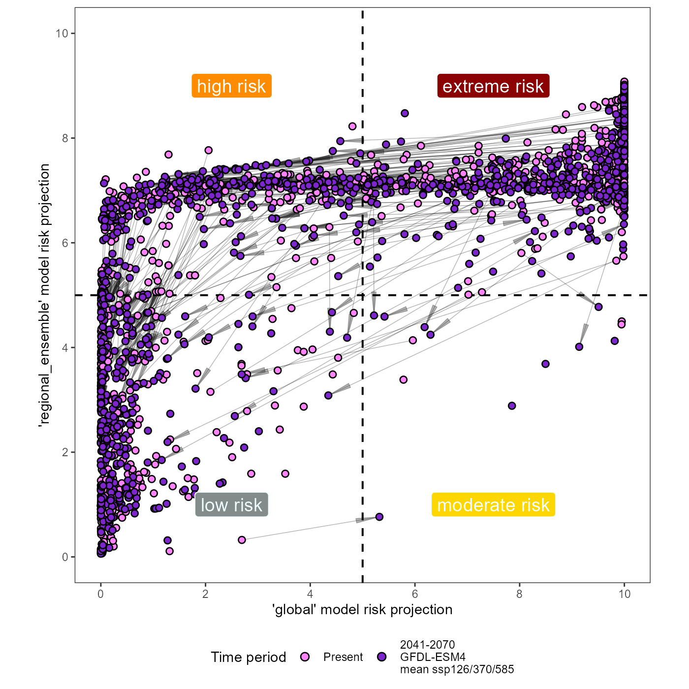

ggsave(
  xy_joined_rescaled_plot, 
  filename = file.path(
    here::here(), "vignette-outputs", "figures", "IVR_risk_plot.jpg"
    ),
  height = 8, 
  width = 8,
  device = jpeg,
  dpi = "retina"
  )

# I will also save the ggplot object as an rds because I need to facet it later
write_rds(
  xy_joined_rescaled_plot,
  file = file.path(here::here(), "vignette-outputs", "figures", "figures-rds", "IVR_risk_plot.rds")
  )

The plot shows the projected change in suitability of our viticultural regions under climate change. The arrows indicate that a region is crossing a suitability value, from being suitable for SLF establishment to being unsuitable.

4. Create summary table of transformed plot

I will now create a summary table to explain the rescaled plots from step 4. The table will depict the quadrant placement of the point in the quadrant plot, both before and after climate change. From this, I will calculate the total number of movements into and out of each quadrant. I will apply the internal function scari::calculate_risk_quadrant().

I will create a summary table of the quadrant placement (and thus the level of risk) for each point in the IVR_locations dataset. I will use calculate_risk_quadrant() to accomplish this.

# edit IVR_locations first
IVR_locations <- IVR_locations %>%
    dplyr::mutate(
      join_col_x = round(x, 5),
      join_col_y = round(y, 4) # rounding to the 1000s (1km) place to prevent overly sensitive exclusions for UTM data
    )

# create dataset and tidy
IVR_locations_joined <- left_join(IVR_locations, xy_joined_rescaled, by = c("ID", "join_col_x", "join_col_y")) %>%
  dplyr::relocate(ID, x, y) %>%
  # remove join cols
  dplyr::select(-c(join_col_x, join_col_y)) 
  
# calculate risk quadrants
IVR_locations_risk <- IVR_locations_joined %>%
  dplyr::mutate(
    risk_1995 = scari::calculate_risk_quadrant(
      suit.x = IVR_locations_joined$xy_global_1995_rescaled,
      suit.y = IVR_locations_joined$xy_regional_ensemble_1995_rescaled,
      thresh.x = global_MTSS, # this threshold remains the same
      thresh.y = regional_ensemble_MTSS_1995
    ),
    risk_2055 = scari::calculate_risk_quadrant(
      suit.x = IVR_locations_joined$xy_global_2055_rescaled,
      suit.y = IVR_locations_joined$xy_regional_ensemble_2055_rescaled,
      thresh.x = global_MTSS,
      thresh.y = regional_ensemble_MTSS_2055
    ),
    risk_shift = stringr::str_c(risk_1995, risk_2055, sep = "-")
  )

# factor levels
risk_levels <- c("extreme", "high", "moderate", "low")

# number of rows in table
n_records <- nrow(IVR_locations_risk)

IVR_risk_table <- IVR_locations_risk %>%
  # create counts and make into acrostic table
  dplyr::group_by(risk_1995, risk_2055) %>%
  dplyr::summarize(count = n()) %>%
  pivot_wider(names_from = risk_2055, values_from = count) %>%
  # tidy
  ungroup()

## `summarise()` has grouped output by 'risk_1995'. You can override using the
## `.groups` argument.

  # add columns that do not exist
  if(!'extreme' %in% names(IVR_risk_table)) IVR_risk_table <- IVR_risk_table %>% tibble::add_column(extreme = 0)
  if(!'high' %in% names(IVR_risk_table)) IVR_risk_table <- IVR_risk_table %>% tibble::add_column(high = 0)
  if(!'moderate' %in% names(IVR_risk_table)) IVR_risk_table <- IVR_risk_table %>% tibble::add_column(moderate = 0)
  if(!'low' %in% names(IVR_risk_table)) IVR_risk_table <- IVR_risk_table %>% tibble::add_column(low = 0)

  # ensure all combinations of risk exist
  if(!'extreme' %in% IVR_risk_table$risk_1995) IVR_risk_table <- IVR_risk_table %>% tibble::add_row(risk_1995 = "extreme", extreme = 0, high = 0, moderate = 0, low = 0)
  if(!'high' %in% IVR_risk_table$risk_1995) IVR_risk_table <- IVR_risk_table %>% tibble::add_row(risk_1995 = "high", extreme = 0, high = 0, moderate = 0, low = 0)
  if(!'moderate' %in% IVR_risk_table$risk_1995) IVR_risk_table <- IVR_risk_table %>% tibble::add_row(risk_1995 = "moderate", extreme = 0, high = 0, moderate = 0, low = 0)
  if(!'low' %in% IVR_risk_table$risk_1995) IVR_risk_table <- IVR_risk_table %>% tibble::add_row(risk_1995 = "low", extreme = 0, high = 0, moderate = 0, low = 0)

IVR_risk_table <- IVR_risk_table %>%
  dplyr::rename("rows_1995_cols_2055" = "risk_1995") %>%
  dplyr::relocate("rows_1995_cols_2055", "extreme", "high", "moderate") %>%
  dplyr::arrange(factor(.$rows_1995_cols_2055, levels = risk_levels)) %>%
  # replace missing categories with 0
  replace(is.na(.), 0) 

# tidy
IVR_risk_table <- IVR_risk_table %>%
  # add totals column
  tibble::add_column("total_present" = rowSums(.[, 2:5])) %>%
  # add row totals
  tibble::add_row(rows_1995_cols_2055 = "total_2055", extreme = colSums(dplyr::select(., 2)), high = colSums(dplyr::select(., 3)), moderate = colSums(dplyr::select(., 4)), low = colSums(dplyr::select(., 5)), total_present = n_records) %>%
  # convert to df
  as.data.frame()

write_csv(IVR_risk_table, file = file.path(here::here(), "vignette-outputs", "data-tables", "IVR_risk_table.csv"))

We now have a table calculating the number of regions per quadrant, before and after climate change!

5. global risk shift vs regional risk shift

I will create a table to sum the number of points in three different groups. My goal is to understand how the regional model adds resolution to our calculation of risk. I will sum the number of points that are suitable in the global model only, unsuitable in the global model only, and unsuitable in the global model / suitable in the regional model. I will repeat this operation for both time periods.

global_regional_risk_shift <- tibble(
  time_period = c(1995, 1995, 1995, 2055, 2055, 2055),
  quadrants = c("quad4_quad2", "quad3_quad1", "quad3", "quad4_quad2", "quad3_quad1", "quad3"),
  risk = c("extreme_moderate", "high_low", "high", "extreme_moderate", "high_low", "high"),
  model_suit = c("global_suit", "global_unsuit", "global_unsuit_regional_suit", "global_suit", "global_unsuit", "global_unsuit_regional_suit"),
  IVR_region_count = c(
    # global suitable 1995
    sum(IVR_locations_joined$xy_global_1995_rescaled >= global_MTSS),
    # global unsuitable 1995
    sum(IVR_locations_joined$xy_global_1995_rescaled < global_MTSS),
    # global unsuitable and regional suitable 1995
    sum(IVR_locations_joined$xy_global_1995_rescaled < global_MTSS & IVR_locations_joined$xy_regional_ensemble_1995_rescaled >= regional_ensemble_MTSS_1995),
    # global suitable 2055
    sum(IVR_locations_joined$xy_global_2055_rescaled >= global_MTSS),
    # global unsuitable 2055
    sum(IVR_locations_joined$xy_global_2055_rescaled < global_MTSS),
    # global unsuitable and regional suitable 2055
    sum(IVR_locations_joined$xy_global_2055_rescaled < global_MTSS & IVR_locations_joined$xy_regional_ensemble_2055_rescaled >= regional_ensemble_MTSS_2055)
  )
)

# total # IVRs
total_IVR <- sum(global_regional_risk_shift[1:2, 5])

global_regional_risk_shift <- dplyr::mutate(
  global_regional_risk_shift, 
  IVR_region_prop = IVR_region_count / total_IVR
  )


# calculate % of unsuit (quad3 and quad 1) that are are in quad3
quad3_risk_prop <- tibble(
  time_period = c("quad3_1995", "quad3_2055"),
  prop_total_unsuit_in_quad3 = c(
    scales::label_percent(accuracy = 0.01) (abs(as.numeric((global_regional_risk_shift[3, 5]) / global_regional_risk_shift[2, 5]))),
    scales::label_percent(accuracy = 0.01) (abs(as.numeric((global_regional_risk_shift[6, 5]) / global_regional_risk_shift[5, 5])))
  )
)



# number and proportion of IVRs shifting with CC
#global_regional_risk_shift_summary <- tibble(
##  "risk_shift" = c("global_unsuit_shift_1995_2055", "quad3_high_shift_diff_1995_2055"),
#  "IVR_region_change_count" = c(
#    as.numeric(global_regional_risk_shift[2, 5]) - as.numeric(global_regional_risk_shift[5, 5]),
#    as.numeric(global_regional_risk_shift[3, 5]) - as.numeric(global_regional_risk_shift[6, 5])
#  ),
#  "IVR_region_change_prop" = c(
#    as.numeric(global_regional_risk_shift[2, 6]) - as.numeric(global_regional_risk_shift[5, 6]),
#    as.numeric(global_regional_risk_shift[3, 6]) - as.numeric(global_regional_risk_shift[6, 6])
#  )
#) %>%
  # make percentages and change signs
#  mutate(
#    IVR_region_change_count = abs(IVR_region_change_count),
 #   IVR_region_change_prop = scales::label_percent(accuracy = 0.01) (abs(IVR_region_change_prop))
#    )

With this analysis, I found that currently, 65.2% of the global IVRs are low risk according to the global model. However, 26% of the total IVRs are specifically in quadrant 3 (high risk). This means that the global model alone would label 693 of the 1074 IVRs as low risk, when in actuality 287 or about 41.4% of these are at high risk for SLF establishment (above the MTSS threshold) when we spatially segment the presence data into an ensemble of regional-scale models. After climate change, 893 of the 1063 IVRs (82%) would be unsuitable if the global model alone were used to describe the risk of SLF. However, 341 or 39.1% of these unsuitable IVRs are still suitable in regional_scale models and thus would be missed by an analysis of risk using only a global-scale model.

This means that our regional-scale ensemble is adding resolution and nuance to our estimation of risk for SLF establishment.

# add %
global_regional_risk_shift <- dplyr::mutate(global_regional_risk_shift, IVR_region_prop = scales::label_percent(accuracy = 0.01) (IVR_region_prop))

# make kable
global_regional_risk_shift <- kable(global_regional_risk_shift, "html", escape = FALSE) %>% 
  kable_styling(bootstrap_options = "striped", full_width = FALSE) %>%
  # standardize col width
  kableExtra::column_spec(1:2, width_min = '4cm') %>%
  kableExtra::add_header_above(., header = c("IVR risk plot quadrant proportions" = 6), bold = TRUE)


# save as .html
kableExtra::save_kable(
  global_regional_risk_shift, 
  file = file.path(here::here(), "vignette-outputs", "figures", "IVR_risk_plot_quadrant_props.html"),
  self_contained = TRUE
  )

# initialize webshot by 
# webshot::install_phantomjs()
# convert to pdf
webshot::webshot(
  url = file.path(here::here(), "vignette-outputs", "figures", "IVR_risk_plot_quadrant_props.html"),
  file = file.path(here::here(), "vignette-outputs", "figures", "IVR_risk_plot_quadrant_props.jpg"),
  zoom = 2
)
  
file.remove(file.path(here::here(), "vignette-outputs", "figures", "IVR_risk_plot_quadrant_props.html"))

6. Save wineries with pred suitability

I will now join the risk levels dataset I have created with the original wineries_tidied dataset and save this. I will also add a count of the risk levels so they can be compared quantitatively. I will code extreme risk = 4, high = 3, moderate = 2, and low = 1. Then, I will subtract the risk level in 1995 from the risk level in 2055 to quantify the change in risk level over time and calculate summary stats.

# add risk level counts
wineries_tidied_suit <- IVR_locations_risk %>%
  dplyr::mutate(
    risk_1995_count = dplyr::case_when(
      risk_1995 == "extreme" ~ 4,
      risk_1995 == "high" ~ 3,
      risk_1995 == "moderate" ~ 2,
      risk_1995 == "low" ~ 1
    ),
    risk_2055_count = dplyr::case_when(
      risk_2055 == "extreme" ~ 4,
      risk_2055 == "high" ~ 3,
      risk_2055 == "moderate" ~ 2,
      risk_2055 == "low" ~ 1
    ),
    risk_shift_count = risk_2055_count - risk_1995_count
  )

# rename columns
wineries_tidied_suit <- wineries_tidied_suit %>%
  dplyr::rename(
    "global_model_suit_hist" = "xy_global_1995_rescaled",
    "regional_ensemble_model_suit_hist" = "xy_regional_ensemble_1995_rescaled",
    "global_model_suit_2041-2070" = "xy_global_2055_rescaled",
    "regional_ensemble_model_suit_2041-2070" = "xy_regional_ensemble_2055_rescaled",
    "risk_level_hist" = "risk_1995",
    "risk_level_2041-2070" = "risk_2055",
    "risk_count_hist" = "risk_1995_count",
    "risk_count_2041-2070" = "risk_2055_count"
  )

# rearrange columns
wineries_tidied_suit <- wineries_tidied_suit %>%
  dplyr::relocate(risk_count_hist, .after = risk_level_hist) %>%
  dplyr::relocate(`risk_count_2041-2070`, .after = `risk_level_2041-2070`) %>%
  dplyr::relocate(risk_shift_count, .after = risk_shift)

# save 
readr::write_csv(
  x = wineries_tidied_suit,
  file = file.path(here::here(), "vignette-outputs", "data-tables", "wineries_tidied_with_suit_risk.csv")
  )

readr::write_rds(
  x = wineries_tidied_suit,
  file = file.path(here::here(), "data", "wineries_tidied_with_suit_risk.rds")
  )

We now have risk quadrant plots and tables that we can use to assess the level of SLF establishment risk to viticulture.

References

Gallien, L., Douzet, R., Pratte, S., Zimmermann, N. E., & Thuiller, W. (2012). Invasive species distribution models – how violating the equilibrium assumption can create new insights. Global Ecology and Biogeography, 21(11), 1126–1136. https://doi.org/10.1111/j.1466-8238.2012.00768.x
Smith, T. 2021, August 11. Evaluating Invasion Stage with SDMs - plantarum.ca. https://plantarum.ca/2021/08/11/invasion-stage/.

Samuel M. Owens¹

2025-08-04

Overview

Setup

load rasters

tidy wineries dataset

import and tidy xy suitability

take mean of global model ssp scenarios

retrieve suitability values for regional_ensemble

take mean of ssps

1. Transform xy suitability

2. Plot untransformed suitability values

3. plot transformed suitability values

4. Create summary table of transformed plot

5. global risk shift vs regional risk shift

6. Save wineries with pred suitability

References

Plot shift in SLF risk to important viticultural regions under climate change

Samuel M. Owens1

2025-08-04

Overview

Setup

load rasters

tidy wineries dataset

import and tidy xy suitability

take mean of global model ssp scenarios

retrieve suitability values for regional_ensemble

take mean of ssps

1. Transform xy suitability

2. Plot untransformed suitability values

3. plot transformed suitability values

4. Create summary table of transformed plot

5. global risk shift vs regional risk shift

6. Save wineries with pred suitability

References

Samuel M. Owens¹