Plot variable importance for all models

Samuel M. Owens¹

2025-08-07

This vignette will plot the variable permutation importance for all models. Variable importance is critical for me to explore because it helps me to identify which environmental factors are most influential to the presence of SLF based on each model. Variable permutation importance is especially important for discerning fundamental differences between the regional-scale models. It will help us to discern whether SLF occupies a fundamentally different climate in different regions. We can also compare the permutation importance across models to discern whether SLF presence in our different regions is driven by the same or different environmental factors.

Finally, the variable perm. importance will tell us if our ensemble of regional-scale models is actually highlighting a different range of climatic factors that is traditionally missed by a global-scale model. The global-scale model is essentially the mean of all data, but this ignores invasion history (SLF has occupied different regions at different times) and the fact that SLF may actually occupy fundamentally different climates in different regions. By modeling these regions separately and ensembling them into a “regional_ensemble” model, we hypothesized this model would emphasize different climatic variables than the global mean model. We also believe that bio 11, which represents winter temperature minimums, will significantly drive our models, and therefore SLF distribution, across regions.

We will plot the variable importance for all models on the same plot for direct comparison.

Setup

# general tools
library(tidyverse)  #data manipulation
library(here) #making directory pathways easier on different instances
# here::here() starts at the root folder of this package.
library(devtools)

# SDMtune and dependencies
library(SDMtune) # main package used to run SDMs
library(dismo) # package underneath SDMtune
library(rJava) # for running MaxEnt
library(plotROC) # plots ROCs

# html tools
library(kableExtra)
library(webshot)
library(webshot2)

mypath <- file.path(here::here() %>% 
                       dirname(),
                     "maxent/models")

ensemble_colors <- c(
  "Rn (native)" = "#4daf4a",
  "Ri.NAmerica" =  "#e41a1c",
  "Ri.Asia" = "#377eb8"
)

Variable importance

First, import the variable importance output from SDMtune.

regional_native_var_imp <- read.csv(file = file.path(mypath, "slf_regional_native_v4", "regional_native_variable_importance.csv"))

regional_invaded_var_imp <- read.csv(file = file.path(mypath, "slf_regional_invaded_v8", "regional_invaded_variable_importance.csv"))

regional_invaded_asian_var_imp <- read.csv(file = file.path(mypath, "slf_regional_invaded_asian_v3", "regional_invaded_asian_variable_importance.csv"))

Next, use a built-in function from SDMtune to get the base plot for each model.

regional_native_var_imp_plot <- SDMtune::plotVarImp(
  df = regional_native_var_imp
) %>%
  ggplot_build()

# change groups
regional_native_var_imp_plot[["data"]][[1]][["x"]] <- c(1, 4, 2, 3)



regional_invaded_var_imp_plot <- SDMtune::plotVarImp(
  df = regional_invaded_var_imp
) %>%
  ggplot_build()

# change groups
regional_invaded_var_imp_plot[["data"]][[1]][["x"]] <- c(1, 2, 3, 4)



regional_invaded_asian_var_imp_plot <- SDMtune::plotVarImp(
  df = regional_invaded_asian_var_imp
) %>%
  ggplot_build()

# change groups
regional_invaded_asian_var_imp_plot[["data"]][[1]][["x"]] <- c(1, 2, 4, 3)

Finally, plot the regional ensemble models.

var_imp_ensemble <- ggplot() +
  # native model data
  geom_col(data = regional_native_var_imp_plot$data[[1]], aes(x = x + 0.2, y = y, fill = "Rn (native)"), color = "black", width = 0.2) +
  # invaded model data
  geom_col(data = regional_invaded_var_imp_plot$data[[1]], aes(x = x, y = y, fill = "Ri.NAmerica"), color = "black", width = 0.2) +
  # invaded_asian model data
  geom_col(data = regional_invaded_asian_var_imp_plot$data[[1]], aes(x = x - 0.2, y = y, fill = "Ri.Asia"), color = "black", width = 0.2) +
  labs(
    title = "Variable Importance for 'regional_ensemble' models",
    x = "",
    y = "Permutation importance"
    ) +
  scale_x_continuous(
    breaks = c(1, 2, 3, 4),
    labels = c("bio 2", "bio 12", "bio 11", "bio 15")
  ) +
  scale_y_continuous(labels = scales::percent) +
    # aes
  theme_bw() +
  scale_fill_manual(
    name = "model",
    values = ensemble_colors,
    aesthetics = "fill"
  ) +
  theme(legend.position = "bottom") +
  coord_flip()

ggsave(
  var_imp_ensemble, 
  filename = file.path(
    here::here(), "vignette-outputs", "figures", "Variable_importance_regional_ensemble.jpg"
    ),
  height = 8, 
  width = 8,
  device = jpeg,
  dpi = "retina"
  )

Now, repeat the same process, but add the global-scale model to the same plot for direct comparison.

global_var_imp <- read.csv(file = file.path(mypath, "slf_global_v4", "global_variable_importance.csv"))

global_var_imp_plot <- SDMtune::plotVarImp(
  df = global_var_imp
) %>%
  ggplot_build()

var_imp_ensemble_global <- ggplot() +
  # native model data
  geom_col(data = global_var_imp_plot$data[[1]], aes(x = x - 0.4, y = y, fill = "global"), color = "black", width = 0.2) +
  # native model data
  geom_col(data = regional_native_var_imp_plot$data[[1]], aes(x = x - 0.2, y = y, fill = "Rn (native)"), color = "black", width = 0.2) +
  # invaded model data
  geom_col(data = regional_invaded_var_imp_plot$data[[1]], aes(x = x, y = y, fill = "Ri.NAmerica"), color = "black", width = 0.2) +
  # invaded_asian model data
  geom_col(data = regional_invaded_asian_var_imp_plot$data[[1]], aes(x = x + 0.2, y = y, fill = "Ri.Asia"), color = "black", width = 0.2) +
  labs(
    title = "Variable Importance for 'regional_ensemble' and 'global' models",
    x = "",
    y = "Permutation importance"
    ) +
  scale_x_continuous(
    breaks = c(1, 2, 3, 4),
    labels = c("bio 2", "bio 12", "bio 11", "bio 15")
  ) +
  scale_y_continuous(labels = scales::percent) +
    # aes
  theme_bw() +
  scale_fill_manual(
    name = "model",
    values = ensemble_colors,
    aesthetics = "fill"
  ) +
  theme(legend.position = "bottom") +
  coord_flip()

var_imp_ensemble_global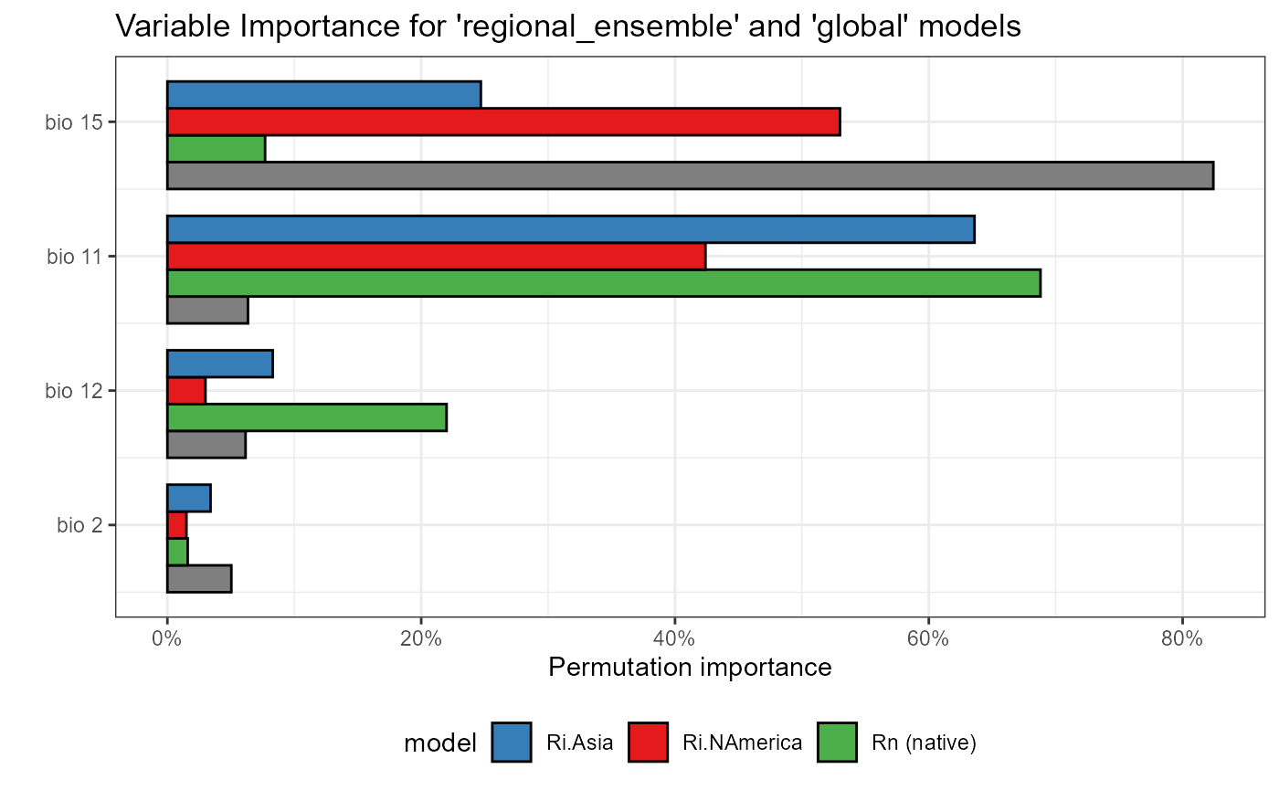

Right off, we can see important differences in the variable importance between the global and regional ensemble models.

The global model emphasizes bio 2 (mean diurnal range) and bio 15 (precipitation seasonality) as the most important variables by far, at about 85%. However, we see that the regional models each disagree on the importance of this variable. The model based on the invaded range in North America agrees that precipitation seasonality is most important, while the Asian invaded and native models each place far less importance on this variable.

Meanwhile, the regional ensemble models all emphasize bio 11 (mean temperature of the coldest quarter) as being of high importance. The N American invaded model places this variable at second, but still sees it as important. The native and invaded Asian models both place this variable as the most important. This suggests that SLF occupies a fundamentally different climate in different regions, which is consistent with our hypothesis that SLF presence is driven by different environmental factors in different regions.

Another of our initial hypotheses was that winter temperature minimums would drive the distribution of SLF, which we are seeing from our regional-scale model. However, we would not see this using only the global mean model, which rates bio 11 as among the least important variables.

Indeed, our regional_ensemble is clarifying important variables we would not have seen with a global mean model.