Assess model goodness of fit via AUC, TSS and confusion matrices

In this vignette, I will assess the fit of my models using a few different metrics: the TSS score, AUC score, and confusion matrices.

First, I will look at the TSS score, which is a threshold-dependent metric of model fit. Considering our decision to convert our risk maps to presence/absence maps using the MTSS threshold, this is an important step. The TSS measures the fit at the threshold where the TSS is maximized (the MTSS threshold).

Next, we will look at the AUC score, which is a threshold-independent metric of model fit. The AUC score is the area under the ROC curve, which is a plot of the true positive rate (sensitivity) against the false positive rate (1 - specificity). The AUC score ranges from 0 to 1, with a score of below 0.5 indicating no discrimination, a score of 0.5 being discrimination equal to a random result, and a score of 1 indicating perfect discrimination. Overall, this test assesses the model’s ability to discriminate a true positive from a false positive.I will plot all four ROC curves on the same plot, allowing for a direct comparison of the AUC (goodness of fit) between models.

Finally, I will look at confusion matrices, which provide a summary of the model’s performance in terms of true positives, false positives, true negatives, and false negatives. These matrices will allow us to calculate sensitivity, specificity, commission error, and omission error for each model.

Setup

# general tools
library(tidyverse)  #data manipulation
library(here) #making directory pathways easier on different instances
# here::here() starts at the root folder of this package.
library(devtools)

# spatial data
library(terra)

# SDMtune and dependencies
library(SDMtune) # main package used to run SDMs
library(dismo) # package underneath SDMtune
library(rJava) # for running MaxEnt
library(plotROC) # plots ROCs

# html tools
library(kableExtra)
library(webshot)
library(webshot2)

These plots depict the activity of the variables put into the MaxEnt models. I will create a combined figure for the 3 models in the regional_ensemble

mypath <- file.path(here::here() %>% 
                       dirname(),
                     "maxent/models")

ensemble_colors <- c(
  "Rn (native)" = "#4daf4a",
  "Ri.NAmerica" =  "#e41a1c",
  "Ri.Asia" = "#377eb8"
)

regional_native_model <- read_rds(file = file.path(mypath, "slf_regional_native_v4", "regional_native_model.rds"))

regional_invaded_model <- read_rds(file = file.path(mypath, "slf_regional_invaded_v8", "regional_invaded_model.rds"))

regional_invaded_asian_model <- read_rds(file = file.path(mypath, "slf_regional_invaded_asian_v3", "regional_invaded_asian_model.rds"))

TSS Score

First, we will assess the TSS score for each model. The TSS score is a measure of the model’s ability to discriminate between presence and absence data, with values ranging from -1 to 1. A value of 0 indicates no discrimination, while a value of 1 indicates perfect discrimination. It is a threshold-dependent measure of accuracy, and we have already calculated the TSS score for each model based on the testing data. I will load those in and display them.

regional_native_tss <- read_csv(file = file.path(mypath, "slf_regional_native_v4", "regional_native_auc_tss.csv")) %>%
  # select test TSS
  dplyr::select(TSS) %>%
  dplyr::slice_tail()

regional_invaded_tss <- read_csv(file = file.path(mypath, "slf_regional_invaded_v8", "regional_invaded_auc_tss.csv")) %>%
  dplyr::select(TSS) %>%
  dplyr::slice_tail()

regional_invaded_asian_tss <- read_csv(file = file.path(mypath, "slf_regional_invaded_asian_v3", "regional_invaded_asian_auc_tss.csv")) %>%
  dplyr::select(TSS) %>%
  dplyr::slice_tail()

tss_scores <- tibble(
  model = c("regional native", "regional invaded NAmerica", "regional invaded Asia"),
  TSS = c(
    regional_native_tss$TSS,
    regional_invaded_tss$TSS,
    regional_invaded_asian_tss$TSS
  )
)

tss_scores

## # A tibble: 3 × 2
##   model                       TSS
##   <chr>                     <dbl>
## 1 regional native           0.992
## 2 regional invaded NAmerica 0.289
## 3 regional invaded Asia     0.824

We can see that the native and invaded Asian models have excellent discriminating power, with TSS scores of 0.99 and 0.82, respectively. The invaded North American model has a TSS score of 0.29, indicating that it’s discriminating power is poor.

Despite the poor performance of some of our regional-scale models, we can have confidence in their performance. During the ensemble process (vignette 110), we took a weighted mean of each of the regional-scale models, which allowed us give higher weight to models that performed better according to the AUC metric, and lower weight to the lower performers. Indeed, the native model contributed 44% of the final model output, the invaded Asian model contributed 34% of the final output, and the invaded North American model only contributed 21% of the final weight. This correlates with our TSS scores.

ROC regional ensemble

Prepare data

First, I will build the SWD objects required by SDMtune::plotROC

regional_native_test <- read_csv(file = file.path(here::here(), "vignette-outputs", "data-tables", "regional_native_test_slf_presences_v4.csv"))

regional_invaded_test <- read_csv(file = file.path(here::here(), "vignette-outputs", "data-tables", "regional_invaded_test_slf_presences_v8.csv"))

regional_invaded_asian_test <- read_csv(file = file.path(here::here(), "vignette-outputs", "data-tables", "regional_invaded_asian_test_slf_presences_v3.csv"))

# background points
a_regional_invaded_background_points <- read.csv(file.path(here::here(), "vignette-outputs", "data-tables", "regional_invaded_background_points_v8.csv"))

a_regional_native_background_points <- read.csv(file.path(here::here(), "vignette-outputs", "data-tables", "regional_native_background_points_v4.csv"))

a_regional_invaded_asian_background_points <- read.csv(file.path(here::here(), "vignette-outputs", "data-tables", "regional_invaded_asian_background_points_v3.csv"))

# path to directory
mypath <- file.path(here::here() %>% 
                       dirname(),
                     "maxent/historical_climate_rasters/chelsa2.1_30arcsec")


# the scale used to make xy predictions
x_global_hist_env_covariates_list <- list.files(path = file.path(mypath, "v1_maxent_10km"), pattern = "\\.asc$", full.names = TRUE) %>%
    grep("bio2_1981-2010_global.asc|bio11_1981-2010_global.asc|bio12_1981-2010_global.asc|bio15_1981-2010_global.asc", ., value = TRUE)

I will create rasters of the environmental covariates, stack and gather summary statistics. I will also shorten their names and exclude possible operators from layer names (for example, using the dash symbol was found to interfere with SDMtune making predictions for tables downstream).

# layer name object. Check order of layers first
env_layer_names <- c("bio11", "bio12", "bio15", "bio2")

# global rasters
# stack env covariates
x_global_hist_env_covariates <- terra::rast(x = x_global_hist_env_covariates_list)

# attributes
nlyr(x_global_hist_env_covariates)

## [1] 4

names(x_global_hist_env_covariates)

## [1] "CHELSA_bio11_1981-2010_V.2.1" "CHELSA_bio12_1981-2010_V.2.1"
## [3] "CHELSA_bio15_1981-2010_V.2.1" "CHELSA_bio2_1981-2010_V.2.1"

minmax(x_global_hist_env_covariates)

##     CHELSA_bio11_1981-2010_V.2.1 CHELSA_bio12_1981-2010_V.2.1
## min                    -62.92475                    0.5181913
## max                     31.26968                 6553.5000000
##     CHELSA_bio15_1981-2010_V.2.1 CHELSA_bio2_1981-2010_V.2.1
## min                     3.722476                     0.50000
## max                   226.363098                    18.85155

# ext(x_global_hist_env_covariates)
# crs(x_global_hist_env_covariates)

# I will change the name of the variables because they are throwing errors in SDMtune
names(x_global_hist_env_covariates) <- env_layer_names
# confirmed- SDMtune doesnt like dashes in column names (it is read as a mathematical operation)

rm(x_global_hist_env_covariates_list)

# invaded asian
regional_invaded_asian_test_SWD <- SDMtune::prepareSWD(
  species = "Lycorma delicatula",
  env = x_global_hist_env_covariates, 
  p = regional_invaded_asian_test, 
  a = a_regional_invaded_asian_background_points,
  verbose = TRUE # print helpful messages
  )

## ℹ Extracting predictor information for presence locations✔ Extracting predictor information for presence locations [2s]
## ℹ Extracting predictor information for absence/background locations✔ Extracting predictor information for absence/background locations [3.3s]

# regional native
regional_native_test_SWD <- SDMtune::prepareSWD(
  species = "Lycorma delicatula",
  env = x_global_hist_env_covariates,
  p = regional_native_test, 
  a = a_regional_native_background_points,
  verbose = TRUE # print helpful messages
  )

## ℹ Extracting predictor information for presence locations✔ Extracting predictor information for presence locations [2.1s]
## ℹ Extracting predictor information for absence/background locations✔ Extracting predictor information for absence/background locations [7s]

# regional invaded
regional_invaded_test_SWD <- SDMtune::prepareSWD(
  species = "Lycorma delicatula",
  env = x_global_hist_env_covariates, 
  p = regional_invaded_test, 
  a = a_regional_invaded_background_points,
  verbose = TRUE # print helpful messages
  )

## ℹ Extracting predictor information for presence locations✔ Extracting predictor information for presence locations [2s]
## ℹ Extracting predictor information for absence/background locations✔ Extracting predictor information for absence/background locations [4.9s]

Plot

Next, I will use SDMtune to build the ROC plots.

regional_native_ROC <- SDMtune::plotROC(
  model = regional_native_model,
  test = regional_native_test_SWD
) %>%
  ggplot_build()

regional_invaded_ROC <- SDMtune::plotROC(
  model = regional_invaded_model,
  test = regional_invaded_test_SWD
) %>%
  ggplot_build()

regional_invaded_asian_ROC <- SDMtune::plotROC(
  model = regional_invaded_asian_model,
  test = regional_invaded_asian_test_SWD
) %>%
  ggplot_build()

ROC_ensemble <- ggplot() +
  # native model data
  geom_line(data = regional_native_ROC$data[[1]], aes(x = x, y = y, color = "Rn (native)", group = group, linetype = as.factor(group)), linewidth = 0.8) +
  # invaded model data
  geom_line(data = regional_invaded_ROC$data[[1]], aes(x = x, y = y, color = "Ri.NAmerica", group = group, linetype = as.factor(group)), linewidth = 0.8) +
  # invaded_asian model data
  geom_line(data = regional_invaded_asian_ROC$data[[1]], aes(x = x, y = y, color = "Ri.Asia", group = group, linetype = as.factor(group)), linewidth = 0.8) +
  # midpoint line
  geom_abline(slope = 1, linetype = "dashed") +
  # scales
  scale_x_continuous(name = "False positive rate (1 - specificity)", breaks = c(0, 0.25, 0.5, 0.75, 1), limits = c(0, 1)) +
  scale_y_continuous(name = "True positive rate (sensitivity)", breaks = c(0, 0.25, 0.5, 0.75, 1), limits = c(0, 1)) +
  labs(
    title = "ROC curve (true vs false positive rate) for 'regional_ensemble' models"
    ) +
  theme_bw() +
  # aes
  scale_color_manual(
    name = "model",
    values = ensemble_colors,
    aesthetics = "color"
  ) +
  scale_linetype_manual(
    name = "Data segment",
    values = c("solid", "dotted"),
    labels = c("Test", "Train"),
    guide = guide_legend(reverse = TRUE)
  ) +
  theme(legend.position = "bottom") +
  coord_fixed(ratio = 1)

ROC_ensemble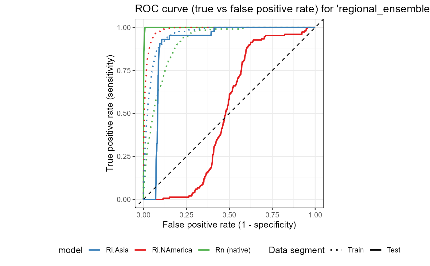

We see that the regional-scale model has the highest testing AUC (0.99), followed by the invaded Asian model (0.90) and finally the invaded North American model (0.51). The invaded North American model is only slightly better than random (0.5), which is consistent with its low TSS score (0.29). Thankfully, however, we have significantly downweighted this model in our ensemble, so it should not have a large impact on our final risk map.

Add global model to ROC plot

Now that I have plotted a separate figure for the three regional_ensemble models, I will create an aggregated figure that includes the ROC plot for all three regional_ensemble models and the global model. This will allow for a direct comparison of the AUC (goodness of fit) between the regional_ensemble and global models.

ROC

mypath <- file.path(here::here() %>% 
                       dirname(),
                     "maxent/models")

# model
global_model <- read_rds(file = file.path(mypath, "slf_global_v4", "global_model.rds"))
# background csv
global_background <- read_csv(file = file.path(here::here(), "vignette-outputs", "data-tables", "global_background_points_v4.csv"))
# all 
slf_points <- readr::read_rds(file = file.path(here::here(), "data", "slf_all_coords_final_2025-07-07.rds")) %>%
  dplyr::select(-species) 

ensemble_colors <- c(
  "Rn (native)" = "#4daf4a",
  "Ri.NAmerica" =  "#e41a1c",
  "Ri.Asia" = "#377eb8",
  "global" = "black"
)

global_SWD <- SDMtune::prepareSWD(
  species = "Lycorma delicatula",
  env = x_global_hist_env_covariates,
  p = slf_points,
  a = global_background,
  verbose = TRUE # print helpful messages
  )

## ℹ Extracting predictor information for presence locations✔ Extracting predictor information for presence locations [3.5s]
## ℹ Extracting predictor information for absence/background locations✔ Extracting predictor information for absence/background locations [13.2s]

# split into train and test sets
global_trainTest <-  SDMtune::trainValTest(
  x = global_SWD,
  test = 0.2, # set used for predicting maps and suitability values
  only_presence = TRUE, # only split presences and recycle bg points
  seed = 3 # should be the same as the OG because same seed
)

# separate off testing data
global_test_SWD <- global_trainTest[[2]]

global_ROC <- SDMtune::plotROC(
  model = global_model@models[[5]], # just pick one because they did not vary too much
  test = global_test_SWD
) %>%
  ggplot_build()

ROC_ensemble_global <- ggplot() +
  # global
  geom_line(data = global_ROC$data[[1]], aes(x = x, y = y, color = "global", group = group, linetype = as.factor(group)), linewidth = 0.8) +
  # native model data
  geom_line(data = regional_native_ROC$data[[1]], aes(x = x, y = y, color = "Rn (native)", group = group, linetype = as.factor(group)), linewidth = 0.8) +
  # invaded model data
  geom_line(data = regional_invaded_ROC$data[[1]], aes(x = x, y = y, color = "Ri.NAmerica", group = group, linetype = as.factor(group)), linewidth = 0.8) +
  # invaded_asian model data
  geom_line(data = regional_invaded_asian_ROC$data[[1]], aes(x = x, y = y, color = "Ri.Asia", group = group, linetype = as.factor(group)), linewidth = 0.8) +
  # midpoint line
  geom_abline(slope = 1, linetype = "dashed") +
  # scales
  scale_x_continuous(name = "False positive rate (1 - specificity)", breaks = c(0, 0.25, 0.5, 0.75, 1), limits = c(0, 1)) +
  scale_y_continuous(name = "True positive rate (sensitivity)", breaks = c(0, 0.25, 0.5, 0.75, 1), limits = c(0, 1)) +
  labs(
    title = "ROC curve (true vs false positive rate) for 'regional_ensemble' and 'global' models"
    ) +
  theme_bw() +
  # aes
  scale_color_manual(
    name = "model",
    values = ensemble_colors,
    aesthetics = "color"
  ) +
  scale_linetype_manual(
    name = "Data segment",
    values = c("solid", "dotted"),
    labels = c("Test", "Train"),
    guide = guide_legend(reverse = TRUE)
  ) +
  theme(legend.position = "bottom") +
  coord_fixed(ratio = 1)

ROC_ensemble_global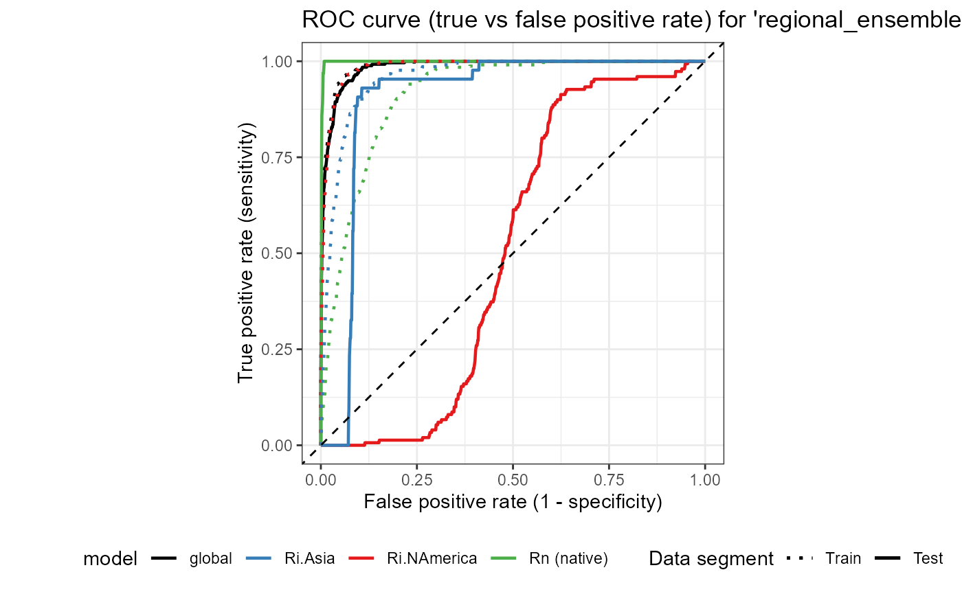

Confusion Matrix- Sensitivity and Specificity of Models

I will create a table for some important summary statistics for the models. These include sensitivity, specificity, commission error, and omission error. These are calculated according to the cloglog MTSS threshold per model.

mypath <- file.path(here::here() %>% 
                       dirname(),
                     "maxent/models")

We calculate these according to the cloglog MTSS threshold per model

# global
global_conf_matr <- read_csv(file = file.path(mypath, "slf_global_v4", "global_thresh_confusion_matrix_all_iterations.csv")) %>%
  # only MTSS threshold
  slice(7)


# regional models
# native
regional_native_conf_matr <- read_csv(file = file.path(mypath, "slf_regional_native_v4", "regional_native_thresh_confusion_matrix.csv")) %>%
  slice(7)
# invaded_asia
regional_invaded_asian_conf_matr <- read_csv(file = file.path(mypath, "slf_regional_invaded_asian_v3", "regional_invaded_asian_thresh_confusion_matrix.csv")) %>%
  slice(7)
# invaded_NAmerica
regional_invaded_conf_matr <- read_csv(file = file.path(mypath, "slf_regional_invaded_v8", "regional_invaded_thresh_confusion_matrix.csv")) %>%
  slice(7)

global_conf_matr

## # A tibble: 1 × 6
##   threshold_type                 threshold_value tp_mean fp_mean fn_mean tn_mean
##   <chr>                                    <dbl>   <dbl>   <dbl>   <dbl>   <dbl>
## 1 Maximum.training.sensitivity.…          0.0169    240.    1307    15.7   18693

I will create some input datasets which contain the number of test positives per model.

global_test_pos <- sum(global_test_SWD@pa == 1)
# regional
regional_native_test_pos <- nrow(regional_native_test)
regional_invaded_test_pos <- nrow(regional_invaded_test)
regional_invaded_asian_test_pos <- nrow(regional_invaded_asian_test)

model_sens_spec <- tibble(
  metric = rep(c("sensitivity", "specificity", "commission error", "omission error"), 4),
  description = rep(c("true_positive rate", "true_negative rate", "1 - true_negative rate", "false_negative rate"), 4),
    model = c(
    rep("global", 4),
    rep("regional native", 4),
    rep("regional invaded NAmerica", 4),
    rep("regional invaded Asia", 4)
  ),
  # cloglog MTSS threshold
  thresh = "MTSS.cloglog",
  thresh_value = c(
    rep(global_conf_matr$threshold_value, 4), 
    rep(regional_native_conf_matr$threshold_value, 4), 
    rep(regional_invaded_conf_matr$threshold_value, 4),
    rep(regional_invaded_asian_conf_matr$threshold_value, 4)
    ),
  # the number of test positives
  test_pos = c(
    rep(global_test_pos, 4), # global, this counts the number of positives in the model (the 1s in the training data)
    rep(regional_native_test_pos, 4),  # native
    rep(regional_invaded_test_pos, 4), # invaded_NAmerica
    rep(regional_invaded_asian_test_pos, 4) # invaded_Asia
  ),
  # the number of background points
  bg_neg = c(
    rep(20000, 4), # global
    rep(10000, 12) # regional
  ),
  value = c(
    # global
    round(global_conf_matr$tp_mean / global_test_pos, 4), # sensitivity (the tp rate)
    round(global_conf_matr$tn_mean / 20000, 4), # specificity (the tn rate)
    round(1 - (global_conf_matr$tn_mean / 20000), 4),  # commission error (1 - tn rate)
    round((global_conf_matr$fn_mean / 20000), 4), # omission error (the fn rate)
    # native
    round(regional_native_conf_matr$tp / regional_native_test_pos, 4), 
    round(regional_native_conf_matr$tn / 10000, 4), 
    round(1 - (regional_native_conf_matr$tn / 10000), 4), 
    round((regional_native_conf_matr$fn / 10000), 4),
    # invaded_NAmerica
    round(regional_invaded_conf_matr$tp / regional_invaded_test_pos, 4), 
    round(regional_invaded_conf_matr$tn / 10000, 4), 
    round(1 - (regional_invaded_conf_matr$tn / 10000), 4), 
    round((regional_invaded_conf_matr$fn / 10000), 4),
    # invaded_asia
    round(regional_invaded_asian_conf_matr$tp / regional_invaded_asian_test_pos, 4), 
    round(regional_invaded_asian_conf_matr$tn / 10000, 4), 
    round(1 - (regional_invaded_asian_conf_matr$tn / 10000), 4), 
    round((regional_invaded_asian_conf_matr$fn / 10000), 4)
  )
)

I will also write it to a kable so it can be printed

# add column formatting
model_sens_spec <- dplyr::mutate(model_sens_spec, bg_neg = scales::label_comma() (bg_neg))

# convert to kable
model_sens_spec_kable <- knitr::kable(x = model_sens_spec, format = "html", escape = FALSE) %>%
  kableExtra::kable_styling(bootstrap_options = "striped", full_width = TRUE)

model_sens_spec_kable

metric	description	model	thresh	thresh_value	test_pos	bg_neg	value
sensitivity	true_positive rate	global	MTSS.cloglog	0.01693	256	20,000	0.9388
specificity	true_negative rate	global	MTSS.cloglog	0.01693	256	20,000	0.9346
commission error	1 - true_negative rate	global	MTSS.cloglog	0.01693	256	20,000	0.0654
omission error	false_negative rate	global	MTSS.cloglog	0.01693	256	20,000	0.0008
sensitivity	true_positive rate	regional native	MTSS.cloglog	0.28320	64	10,000	1.0000
specificity	true_negative rate	regional native	MTSS.cloglog	0.28320	64	10,000	0.7745
commission error	1 - true_negative rate	regional native	MTSS.cloglog	0.28320	64	10,000	0.2255
omission error	false_negative rate	regional native	MTSS.cloglog	0.28320	64	10,000	0.0000
sensitivity	true_positive rate	regional invaded NAmerica	MTSS.cloglog	0.07810	150	10,000	0.0000
specificity	true_negative rate	regional invaded NAmerica	MTSS.cloglog	0.07810	150	10,000	0.9319
commission error	1 - true_negative rate	regional invaded NAmerica	MTSS.cloglog	0.07810	150	10,000	0.0681
omission error	false_negative rate	regional invaded NAmerica	MTSS.cloglog	0.07810	150	10,000	0.0150
sensitivity	true_positive rate	regional invaded Asia	MTSS.cloglog	0.10970	43	10,000	0.9302
specificity	true_negative rate	regional invaded Asia	MTSS.cloglog	0.10970	43	10,000	0.8712
commission error	1 - true_negative rate	regional invaded Asia	MTSS.cloglog	0.10970	43	10,000	0.1288
omission error	false_negative rate	regional invaded Asia	MTSS.cloglog	0.10970	43	10,000	0.0003

We see once again that all models have adequate sensitivity and specificity, but the outlier is the invaded North American model. This model actually had a sensitivity of 0, which means it did not detect any of its test points. The testing range for this model was the invaded range in Asia, where the model predicted no area of suitability above the MTSS threshold. This is likely due to the significant difference in precipitation seasonality. The current invaded North American range has a very narrow range of precipitation seasonality, as compared with the test area in Korea and Japan, which have seasonal monsoons. You can observe this by looking at the variable curve for bio 15; the invaded asian and North American models occupied entirely different ranges of precipitation seasonality. Thus, the training range likely did not translate well to the testing range in Asia.

Otherwise, all models have an adequate fit. The ensemble accounts for the bad fit of the North American model, which we will continue to include due to the potential for this range to expand over time and the important data it includes.

References

Allouche, O., Tsoar, A., & Kadmon, R. (2006). Assessing the accuracy of species distribution models: Prevalence, kappa and the true skill statistic (TSS). Journal of Applied Ecology, 43(6), 1223–1232. https://doi.org/10.1111/j.1365-2664.2006.01214.x
Jiménez‐Valverde, A. (2012). Insights into the area under the receiver operating characteristic curve (AUC) as a discrimination measure in species distribution modelling. Global Ecology and Biogeography, 21(4), 498–507. https://doi.org/10.1111/j.1466-8238.2011.00683.x
Zou, K. H., O’Malley, A. J., & Mauri, L. (2007). Receiver-Operating Characteristic Analysis for Evaluating Diagnostic Tests and Predictive Models. Circulation, 115(5), 654–657. https://doi.org/10.1161/CIRCULATIONAHA.105.594929

Samuel M. Owens¹

2025-08-05

Setup

TSS Score

ROC regional ensemble

Prepare data

Plot

Add global model to ROC plot

ROC

Confusion Matrix- Sensitivity and Specificity of Models

References

Assess model goodness of fit via AUC, TSS and confusion matrices

Samuel M. Owens1

2025-08-05

Setup

TSS Score

ROC regional ensemble

Prepare data

Plot

Add global model to ROC plot

ROC

Confusion Matrix- Sensitivity and Specificity of Models

References

Samuel M. Owens¹