Analyze biological realism of model response curves

Overview

In this vignette, I will plot the marginal and univariate response curves for the global and each of the regional-scale models. These plots will help me to explore the biological realism of our modeled scales.

I hypothesized that the regional models would have more nuanced responses to the environmental variables than the global model, so these plots will allow me to explore the differences in response curves between these models. These regional models should more closely evaluated because the regional models are trained on a smaller subset of the global data, and thus may be more sensitive to the range of our covariates present in each region.

Note for unsmoothed versions of the same curves, simply change the geom_smooth functions to geom_line and remove the se and method arguments.

Setup

I will start by loading the necessary packages, setting the working directory, and defining some style objects for the plots.

# general tools
library(tidyverse)  #data manipulation
library(here) #making directory pathways easier on different instances
# here::here() starts at the root folder of this package.
library(devtools)

# SDMtune and dependencies
library(SDMtune) # main package used to run SDMs
library(dismo) # package underneath SDMtune
library(rJava)
library(plotROC) # plots ROCs

# spatial data handling
library(raster) 
library(terra) 
library(sf)

library(viridis)
library(patchwork)

Note: I will be setting the global options of this document so that only certain code chunks are rendered in the final .html file. I will set the eval = FALSE so that none of the code is re-run (preventing files from being overwritten during knitting) and will simply overwrite this in chunks with plots.

These plots depict the activity of the variables put into the MaxEnt models. I will create a combined figure for the 3 models in the regional_ensemble

mypath <- file.path(here::here() %>% 
                       dirname(),
                     "maxent/models")

Lastly, load in the model objects for plotting the curves.

regional_native_model <- read_rds(file = file.path(mypath, "slf_regional_native_v4", "regional_native_model.rds"))

regional_invaded_model <- read_rds(file = file.path(mypath, "slf_regional_invaded_v8", "regional_invaded_model.rds"))

regional_invaded_asian_model <- read_rds(file = file.path(mypath, "slf_regional_invaded_asian_v3", "regional_invaded_asian_model.rds"))

This vignette contains 3 main types of code chunks, which can be discerned by the title:

Extract ___ plots per model: This type of chunk extracts different types of response curves per model and environmental variable.
Maximum Activity: This type of chunk extracts the value of the maximum activity of the model along the curve for plotting
Combine Plots: This type of chunk combines the plots of the models response curves, per environmental variable and separately for the regional-scale and global-scale models.

The first section of the code performs these operations for the regional-scale models (both univariate and marginal) and the second part creates plots of the same curves but for the global-scale model.

We will focus on the univariate curves, so you will not see the code for the marginal response plots in the rendered version.

1. create univariate response curves- regional_ensemble models

I will smooth these plots using a GAM formula, after the methods of Elith et al, 2011. Note that these curves were created using a Beta multiplier of 1.5.

First, I will create the plotting objects I need.

ensemble_colors <- c(
  "Rn (native)" = "#4daf4a",
  "Ri.NAmerica" =  "#e41a1c",
  "Ri.Asia" = "#377eb8"
)

univar_plots_style <- list(
  theme_bw(),
  # labs
  labs(
    title = "Univariate response in 'regional_ensemble' models",
    color = "Model",
    caption = "rug plots indicate presences"
    ),
  ylab("cloglog_output"),
  # aes
  scale_color_manual(
    name = "model",
    values = ensemble_colors,
    aesthetics = "color"
  ),
  scale_y_continuous(breaks = c(0, 0.25, 0.5, 0.75, 1), limits = c(0, 1)),
  theme(legend.position = "bottom"),
  geom_hline(aes(yintercept = 0), color = "black", linewidth = 0.5) 
)

Bio 11- Mean temperature of the coldest Quarter

regional_native_univar_bio11 <- SDMtune::plotResponse(
  model = regional_native_model,
  var = "bio11",
  type = "cloglog",
  fun = mean,
  only_presence = TRUE,
  marginal = FALSE,
  rug = TRUE
) %>%
  ggplot_build()


regional_invaded_univar_bio11 <- SDMtune::plotResponse(
  model = regional_invaded_model,
  var = "bio11",
  type = "cloglog",
  fun = mean,
  only_presence = TRUE,
  marginal = FALSE,
  rug = TRUE
) %>%
  ggplot_build()

regional_invaded_asian_univar_bio11 <- SDMtune::plotResponse(
  model = regional_invaded_asian_model,
  var = "bio11",
  type = "cloglog",
  fun = mean,
  only_presence = TRUE,
  marginal = FALSE,
  rug = TRUE
) %>%
  ggplot_build()

# peak y trendline object 
bio11_univar_max_activity_values <- c(
  native_bio11 = regional_native_univar_bio11$data[[1]][which.max(regional_native_univar_bio11$data[[1]]$y), ]$x,
  invaded_bio11 = regional_invaded_univar_bio11$data[[1]][which.max(regional_invaded_univar_bio11$data[[1]]$y), ]$x,
  invaded_asian_bio11 = regional_invaded_asian_univar_bio11$data[[1]][which.max(regional_invaded_asian_univar_bio11$data[[1]]$y), ]$x
)

bio11_univar_combined <- ggplot() +
  # native model data
  geom_smooth(data = regional_native_univar_bio11$data[[1]], aes(x = x, y = y, color = "Rn (native)"), se = FALSE, method = "gam") +
  # invaded model data
  geom_smooth(data = regional_invaded_univar_bio11$data[[1]], aes(x = x, y = y, color = "Ri.NAmerica"), se = FALSE, method = "gam") +
  # Ri.Asia model data
  geom_smooth(data = regional_invaded_asian_univar_bio11$data[[1]], aes(x = x, y = y, color = "Ri.Asia"), se = FALSE, method = "gam") +
  # plot peak trendline and labels
  # Rn (native)
  geom_vline(aes(xintercept = bio11_univar_max_activity_values[[1]], color = "Rn (native)"), linetype = "dashed", linewidth = 0.5) +
  # invaded
  geom_vline(aes(xintercept = bio11_univar_max_activity_values[[2]], color = "Ri.NAmerica"), linetype = "dashed", linewidth = 0.5) +
  # Ri.Asia
  geom_vline(aes(xintercept = bio11_univar_max_activity_values[[3]], color = "Ri.Asia"), linetype = "dashed", linewidth = 0.5) +
  # plot rug plots
  # Rn (native)
  geom_rug(aes(x = regional_native_univar_bio11$data[[2]]$x, color = "Rn (native)"), sides = "t") +
  # invaded
  geom_rug(aes(x = regional_invaded_univar_bio11$data[[2]]$x, color = "Ri.NAmerica"), sides = "t", alpha = 0.8) +
  # Ri.Asia
  geom_rug(aes(x = regional_invaded_asian_univar_bio11$data[[2]]$x, color = "Ri.Asia"), sides = "t", alpha = 0.6) +
  # default style
  univar_plots_style +
  # labels
  labs(
    subtitle = "Bio 11 (mean temperature of the coldest quarter)",
    x = "mean temperature of the coldest quarter (C)"
    ) +
  # aesthetics
  xlim(-20, 20) 
  
bio11_univar_combined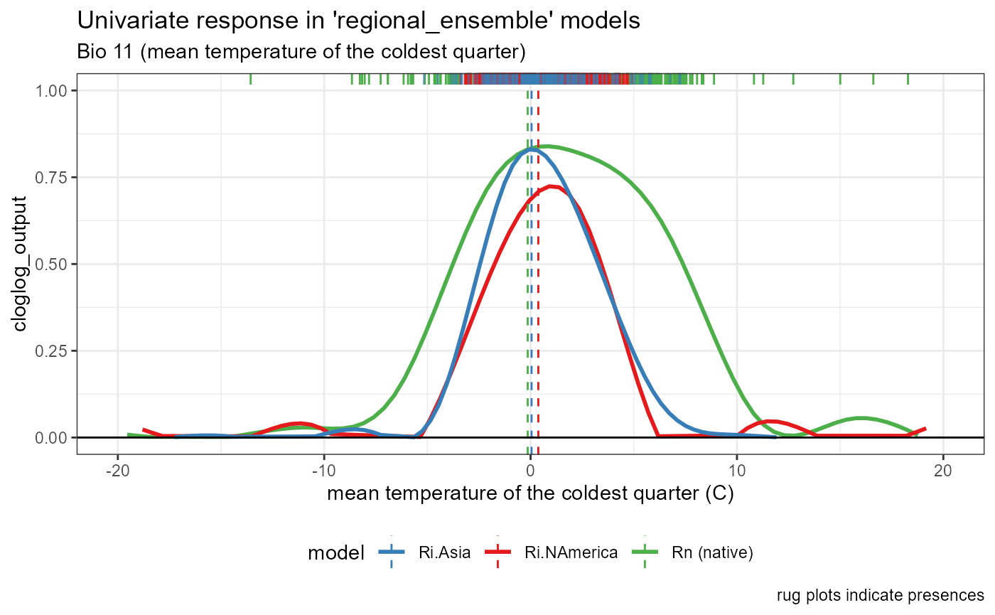

Bio 12- Annual Precipitation

regional_native_univar_bio12 <- SDMtune::plotResponse(
  model = regional_native_model,
  var = "bio12",
  type = "cloglog",
  fun = mean,
  only_presence = TRUE,
  marginal = FALSE,
  rug = TRUE
) %>%
  ggplot_build()


regional_invaded_univar_bio12 <- SDMtune::plotResponse(
  model = regional_invaded_model,
  var = "bio12",
  type = "cloglog",
  fun = mean,
  only_presence = TRUE,
  marginal = FALSE,
  rug = TRUE
) %>%
  ggplot_build()

regional_invaded_asian_univar_bio12 <- SDMtune::plotResponse(
  model = regional_invaded_asian_model,
  var = "bio12",
  type = "cloglog",
  fun = mean,
  only_presence = TRUE,
  marginal = FALSE,
  rug = TRUE
) %>%
  ggplot_build()

# peak y trendline object 
bio12_univar_max_activity_values <- c(
  native_bio12 = regional_native_univar_bio12$data[[1]][which.max(regional_native_univar_bio12$data[[1]]$y), ]$x,
  invaded_bio12 = regional_invaded_univar_bio12$data[[1]][which.max(regional_invaded_univar_bio12$data[[1]]$y), ]$x,
  invaded_asian_bio12 = regional_invaded_asian_univar_bio12$data[[1]][which.max(regional_invaded_asian_univar_bio12$data[[1]]$y), ]$x
)

bio12_univar_combined <- ggplot() +
  # native model data
  geom_smooth(data = regional_native_univar_bio12$data[[1]], aes(x = x, y = y, color = "Rn (native)"), se = FALSE, method = "gam") +
  # invaded model data
  geom_smooth(data = regional_invaded_univar_bio12$data[[1]], aes(x = x, y = y, color = "Ri.NAmerica"), se = FALSE, method = "gam") +
  # invaded_asian model data
  geom_smooth(data = regional_invaded_asian_univar_bio12$data[[1]], aes(x = x, y = y, color = "Ri.Asia"), se = FALSE, method = "gam") +
  # plot peak trendline and labels
  # Rn (native)
  geom_vline(aes(xintercept = bio12_univar_max_activity_values[[1]], color = "Rn (native)"), linetype = "dashed", linewidth = 0.5) +
  # invaded
  geom_vline(aes(xintercept = bio12_univar_max_activity_values[[2]], color = "Ri.NAmerica"), linetype = "dashed", linewidth = 0.5) +
  # Ri.Asia
  geom_vline(aes(xintercept = bio12_univar_max_activity_values[[3]], color = "Ri.Asia"), linetype = "dashed", linewidth = 0.5) +
  # plot rug plots
  # Rn (native)
  geom_rug(aes(x = regional_native_univar_bio12$data[[2]]$x, color = "Rn (native)"), sides = "t") +
  # invaded
  geom_rug(aes(x = regional_invaded_univar_bio12$data[[2]]$x, color = "Ri.NAmerica"), sides = "t", alpha = 0.8) +
  # Ri.Asia
  geom_rug(aes(x = regional_invaded_asian_univar_bio12$data[[2]]$x, color = "Ri.Asia"), sides = "t", alpha = 0.6) +
  # default style
  univar_plots_style +
  # labels
  labs(
    subtitle = "Bio 12 (Annual Precipitation)",
    x = "annual precipitation (mm)"
    ) +
  # aesthetics
  xlim(0, 4250) 
  
bio12_univar_combined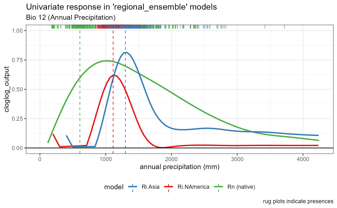

Bio 15- Precipitation Seasonality

regional_native_univar_bio15 <- SDMtune::plotResponse(
  model = regional_native_model,
  var = "bio15",
  type = "cloglog",
  fun = mean,
  only_presence = TRUE,
  marginal = FALSE,
  rug = TRUE
) %>%
  ggplot_build()


regional_invaded_univar_bio15 <- SDMtune::plotResponse(
  model = regional_invaded_model,
  var = "bio15",
  type = "cloglog",
  fun = mean,
  only_presence = TRUE,
  marginal = FALSE,
  rug = TRUE
) %>%
  ggplot_build()

regional_invaded_asian_univar_bio15 <- SDMtune::plotResponse(
  model = regional_invaded_asian_model,
  var = "bio15",
  type = "cloglog",
  fun = mean,
  only_presence = TRUE,
  marginal = FALSE,
  rug = TRUE
) %>%
  ggplot_build()

# peak y trendline object 
bio15_univar_max_activity_values <- c(
  native_bio15 = regional_native_univar_bio15$data[[1]][which.max(regional_native_univar_bio15$data[[1]]$y), ]$x,
  invaded_bio15 = regional_invaded_univar_bio15$data[[1]][which.max(regional_invaded_univar_bio15$data[[1]]$y), ]$x,
  invaded_asian_bio15 = regional_invaded_asian_univar_bio15$data[[1]][which.max(regional_invaded_asian_univar_bio15$data[[1]]$y), ]$x
)

bio15_univar_combined <- ggplot() +
  # native model data
  geom_smooth(data = regional_native_univar_bio15$data[[1]], aes(x = x, y = y, color = "Rn (native)"), se = FALSE, method = "gam") +
  # invaded model data
  geom_smooth(data = regional_invaded_univar_bio15$data[[1]], aes(x = x, y = y, color = "Ri.NAmerica"), se = FALSE, method = "gam") +
  # invaded_asian model data
  geom_smooth(data = regional_invaded_asian_univar_bio15$data[[1]], aes(x = x, y = y, color = "Ri.Asia"), se = FALSE, method = "gam") +
  # plot peak trendline and labels
  # Rn (native)
  geom_vline(aes(xintercept = bio15_univar_max_activity_values[[1]], color = "Rn (native)"), linetype = "dashed", linewidth = 0.5) +
  # invaded
  geom_vline(aes(xintercept = bio15_univar_max_activity_values[[2]], color = "Ri.NAmerica"), linetype = "dashed", linewidth = 0.5) +
  # Ri.Asia
  geom_vline(aes(xintercept = bio15_univar_max_activity_values[[3]], color = "Ri.Asia"), linetype = "dashed", linewidth = 0.5) +
  # plot rug plots
  # Rn (native)
  geom_rug(aes(x = regional_native_univar_bio15$data[[2]]$x, color = "Rn (native)"), sides = "t") +
  # invaded
  geom_rug(aes(x = regional_invaded_univar_bio15$data[[2]]$x, color = "Ri.NAmerica"), sides = "t", alpha = 0.8) +
  # Ri.Asia
  geom_rug(aes(x = regional_invaded_asian_univar_bio15$data[[2]]$x, color = "Ri.Asia"), sides = "t", alpha = 0.6) +
  # default style
  univar_plots_style +
  # labels
  labs(
    subtitle = "Bio 15 (Precipitation Seasonality, CV)",
    x = "precipitation seasonality (%)"
    ) +
  # aesthetics
  xlim(0, 120) 
  
bio15_univar_combined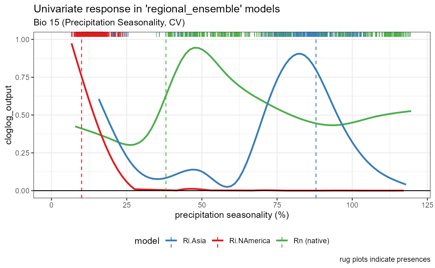

Bio 2- Mean Daily Diurnal Temperature Range

regional_native_univar_bio2 <- SDMtune::plotResponse(
  model = regional_native_model,
  var = "bio2",
  type = "cloglog",
  fun = mean,
  only_presence = TRUE,
  marginal = FALSE,
  rug = TRUE
) %>%
  ggplot_build()


regional_invaded_univar_bio2 <- SDMtune::plotResponse(
  model = regional_invaded_model,
  var = "bio2",
  type = "cloglog",
  fun = mean,
  only_presence = TRUE,
  marginal = FALSE,
  rug = TRUE
) %>%
  ggplot_build()

regional_invaded_asian_univar_bio2 <- SDMtune::plotResponse(
  model = regional_invaded_asian_model,
  var = "bio2",
  type = "cloglog",
  fun = mean,
  only_presence = TRUE,
  marginal = FALSE,
  rug = TRUE
) %>%
  ggplot_build()

# peak y trendline object 
bio2_univar_max_activity_values <- c(
  native_bio2 = regional_native_univar_bio2$data[[1]][which.max(regional_native_univar_bio2$data[[1]]$y), ]$x,
  invaded_bio2 = regional_invaded_univar_bio2$data[[1]][which.max(regional_invaded_univar_bio2$data[[1]]$y), ]$x,
  invaded_asian_bio2 = regional_invaded_asian_univar_bio2$data[[1]][which.max(regional_invaded_asian_univar_bio2$data[[1]]$y), ]$x
)

bio2_univar_combined <- ggplot() +
  # native model data
  geom_smooth(data = regional_native_univar_bio2$data[[1]], aes(x = x, y = y, color = "Rn (native)"), se = FALSE, method = "gam") +
  # invaded model data
  geom_smooth(data = regional_invaded_univar_bio2$data[[1]], aes(x = x, y = y, color = "Ri.NAmerica"), se = FALSE, method = "gam") +
  # Ri.Asia model data
  geom_smooth(data = regional_invaded_asian_univar_bio2$data[[1]], aes(x = x, y = y, color = "Ri.Asia"), se = FALSE, method = "gam") +
  # plot peak trendline and labels
  # Rn (native)
  geom_vline(aes(xintercept = bio2_univar_max_activity_values[[1]], color = "Rn (native)"), linetype = "dashed", linewidth = 0.5) +
  # invaded
  geom_vline(aes(xintercept = bio2_univar_max_activity_values[[2]], color = "Ri.NAmerica"), linetype = "dashed", linewidth = 0.5) +
  # Ri.Asia
  geom_vline(aes(xintercept = bio2_univar_max_activity_values[[3]], color = "Ri.Asia"), linetype = "dashed", linewidth = 0.5) +
  # plot rug plots
  # Rn (native)
  geom_rug(aes(x = regional_native_univar_bio2$data[[2]]$x, color = "Rn (native)"), sides = "t") +
  # invaded
  geom_rug(aes(x = regional_invaded_univar_bio2$data[[2]]$x, color = "Ri.NAmerica"), sides = "t", alpha = 0.8) +
  # Ri.Asia
  geom_rug(aes(x = regional_invaded_asian_univar_bio2$data[[2]]$x, color = "Ri.Asia"), sides = "t", alpha = 0.6) +
  # default style
  univar_plots_style +
  # labels
  labs(
    subtitle = "Bio 2 (Mean Daily Diurnal Temperature Range)",
    x = "mean diurnal range (C)"
    ) +
  # aesthetics
  xlim(0, 15) 
  
bio2_univar_combined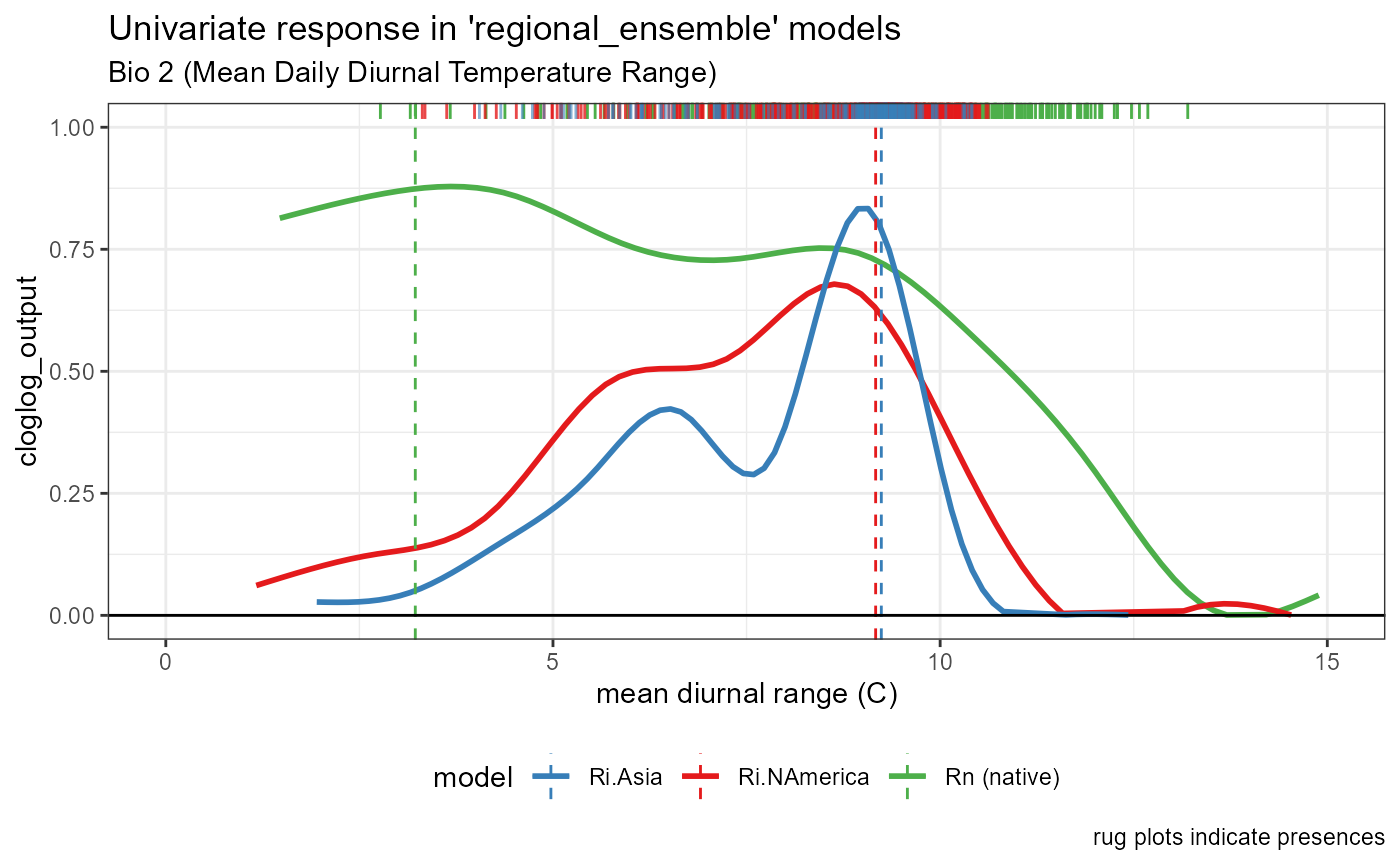

Global Model

Load in objects and setup

univar_plots_style_global <- list(
  theme_bw(),
  # labs
  labs(
    title = "Univariate response of 'global' model",
    caption = "rug plot indicates presences"
    ),
  ylab("cloglog_output"),
  # aes
  scale_y_continuous(breaks = c(0, 0.25, 0.5, 0.75, 1), limits = c(0, 1)),
  geom_hline(aes(yintercept = 0), color = "black", linewidth = 0.5) 
)

global_model <- read_rds(file = file.path(mypath, "slf_global_v4", "global_model.rds"))

Create univariate plots

global_univar_bio11 <- SDMtune::plotResponse(
  model = global_model,
  var = "bio11",
  type = "cloglog",
  fun = mean,
  only_presence = TRUE,
  marginal = FALSE,
  rug = TRUE
) %>%
  ggplot_build()


global_univar_bio12 <- SDMtune::plotResponse(
  model = global_model,
  var = "bio12",
  type = "cloglog",
  fun = mean,
  only_presence = TRUE,
  marginal = FALSE,
  rug = TRUE
) %>%
  ggplot_build()

global_univar_bio15 <- SDMtune::plotResponse(
  model = global_model,
  var = "bio15",
  type = "cloglog",
  fun = mean,
  only_presence = TRUE,
  marginal = FALSE,
  rug = TRUE
) %>%
  ggplot_build()
           

global_univar_bio2 <- SDMtune::plotResponse(
  model = global_model,
  var = "bio2",
  type = "cloglog",
  fun = mean,
  only_presence = TRUE,
  marginal = FALSE,
  rug = TRUE
) %>%
  ggplot_build()

# peak y trendline object 
bio11_univar_max_activity_global <- global_univar_bio11$data[[1]][which.max(global_univar_bio11$data[[1]]$y), ]$x

bio12_univar_max_activity_global <- global_univar_bio12$data[[1]][which.max(global_univar_bio12$data[[1]]$y), ]$x

bio15_univar_max_activity_global <- global_univar_bio15$data[[1]][which.max(global_univar_bio15$data[[1]]$y), ]$x

bio2_univar_max_activity_global <- global_univar_bio2$data[[1]][which.max(global_univar_bio2$data[[1]]$y), ]$x

plots

bio11_univar_global <- ggplot() +
  geom_smooth(data = global_univar_bio11$data[[1]], aes(x = x, y = y), color = "orangered2", se = FALSE, method = "gam") +
  # plot peak trendline and labels
  geom_vline(aes(xintercept = bio11_univar_max_activity_global), color = "orangered2", linetype = "dashed", linewidth = 0.5) +
  # plot rug
  geom_rug(aes(x = global_univar_bio11$data[[3]]$x), color = "orangered2", sides = "t") +
  # default style
  univar_plots_style_global +
  # labels
  # labels
  labs(
    subtitle = "Bio 11 (mean temperature of the coldest quarter)",
    x = "mean temperature of the coldest quarter (C)"
    ) +
  # aesthetics
  xlim(-20, 20)

bio11_univar_global

## `geom_smooth()` using formula = 'y ~ s(x, bs = "cs")'

## Warning: Removed 58 rows containing non-finite outside the scale range
## (`stat_smooth()`).

## Warning: Removed 15 rows containing missing values or values outside the scale range
## (`geom_smooth()`).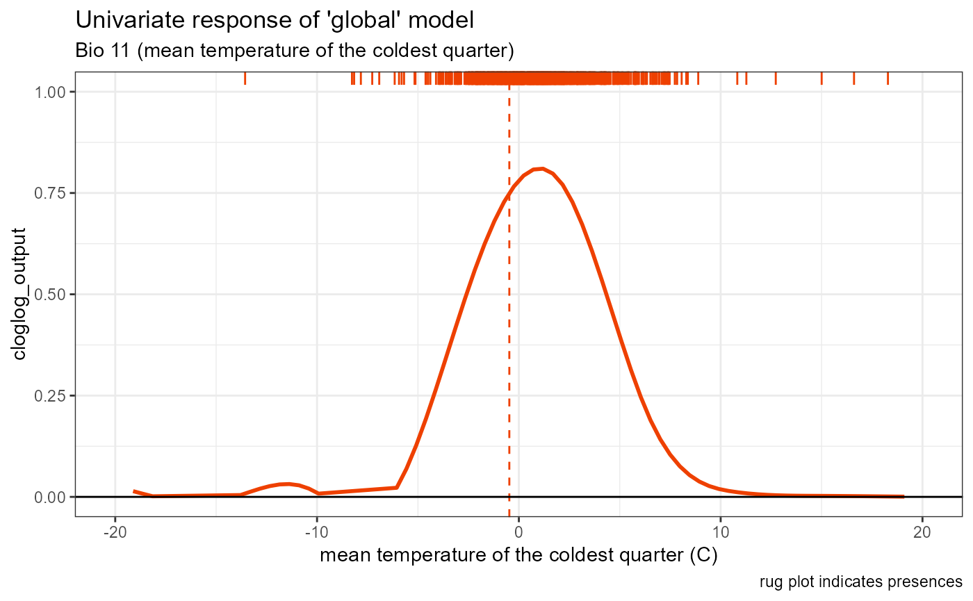

bio12_univar_global <- ggplot() +
  geom_smooth(data = global_univar_bio12$data[[1]], aes(x = x, y = y), color = "orangered2", se = FALSE, method = "gam") +
  # plot peak trendline and labels
  geom_vline(aes(xintercept = bio12_univar_max_activity_global), color = "orangered2", linetype = "dashed", linewidth = 0.5) +
  # plot rug
  geom_rug(aes(x = global_univar_bio12$data[[3]]$x), color = "orangered2", sides = "t") +
  # default style
  univar_plots_style_global +
  # labels
  # labels
  labs(
    subtitle = "Bio 12 (Annual Precipitation)",
    x = "annual precipitation (mm)"
    ) +
  # aesthetics
  xlim(0, 4250)

bio12_univar_global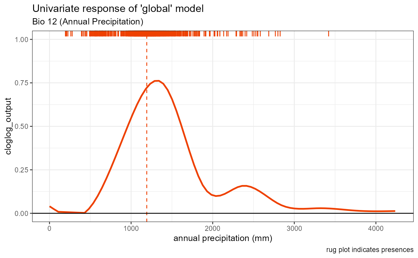

bio15_univar_global <- ggplot() +
  geom_smooth(data = global_univar_bio15$data[[1]], aes(x = x, y = y), color = "orangered2", se = FALSE, method = "gam") +
  # plot peak trendline and labels
  geom_vline(aes(xintercept = bio15_univar_max_activity_global), color = "orangered2", linetype = "dashed", linewidth = 0.5) +
  # plot rug
  geom_rug(aes(x = global_univar_bio15$data[[3]]$x), color = "orangered2", sides = "t") +
  # default style
  univar_plots_style_global +
  # labels
  labs(
    subtitle = "Bio 15 (Precipitation Seasonality, CV)",
    x = "precipitation seasonality (%)"
    ) +
  # aesthetics
  xlim(0, 120) 

bio15_univar_global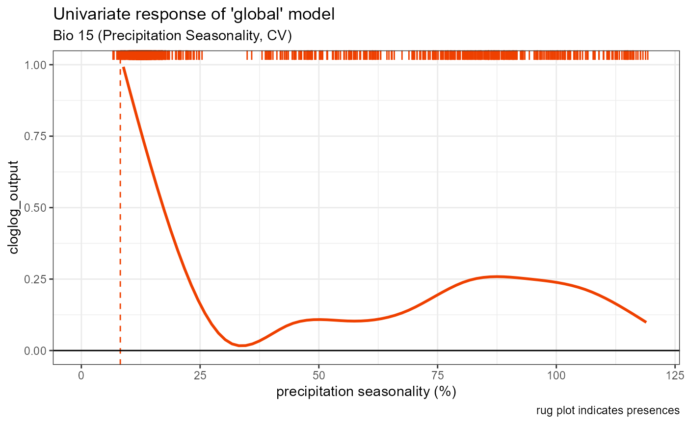

bio2_univar_global <- ggplot() +
  geom_smooth(data = global_univar_bio2$data[[1]], aes(x = x, y = y), color = "orangered2", se = FALSE, method = "gam") +
  # plot peak trendline and labels
  geom_vline(aes(xintercept = bio2_univar_max_activity_global), color = "orangered2", linetype = "dashed", linewidth = 0.5) +
  # plot rug
  geom_rug(aes(x = global_univar_bio2$data[[3]]$x), color = "orangered2", sides = "t") +
  # default style
  univar_plots_style_global +
  # labels
  labs(
    subtitle = "Bio 2 (Mean Diurnal Range)",
    x = "mean diurnal range (C)"
    ) +
  # aesthetics
  xlim(0, 15) 

bio2_univar_global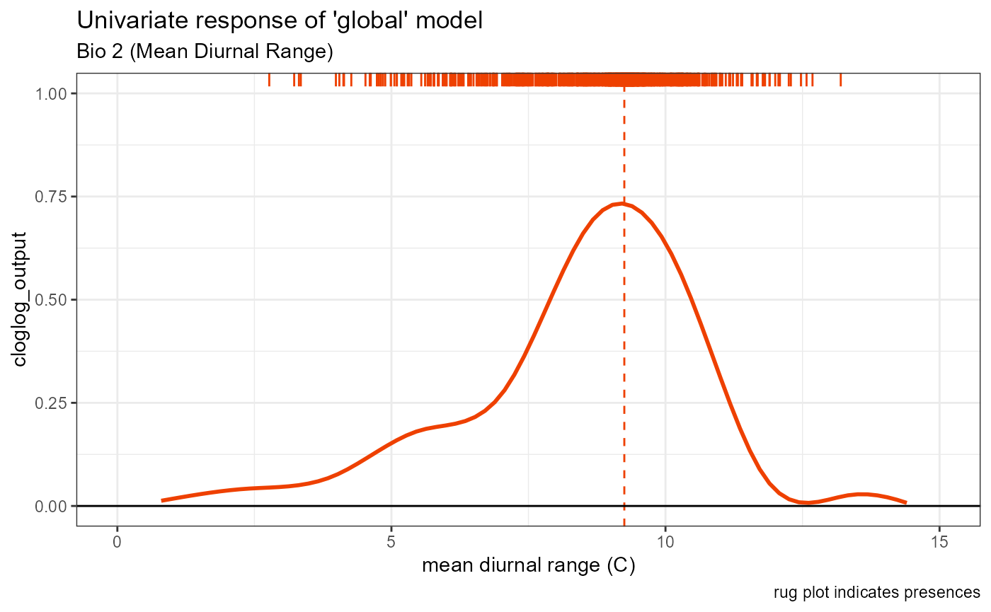

References

Elith, J., Kearney, M., & Phillips, S. (2010). The art of modelling range-shifting species. Methods in Ecology and Evolution, 1(4), 330–342. https://doi.org/10.1111/j.2041-210X.2010.00036.x

Samuel M. Owens¹

2025-08-05

Overview

Setup

1. create univariate response curves- regional_ensemble models

Bio 11- Mean temperature of the coldest Quarter

Bio 12- Annual Precipitation

Bio 15- Precipitation Seasonality

Bio 2- Mean Daily Diurnal Temperature Range

Global Model

Load in objects and setup

Create univariate plots

plots

References

Analyze biological realism of model response curves

Samuel M. Owens1

2025-08-05

Overview

Setup

1. create univariate response curves- regional_ensemble models

Bio 11- Mean temperature of the coldest Quarter

Bio 12- Annual Precipitation

Bio 15- Precipitation Seasonality

Bio 2- Mean Daily Diurnal Temperature Range

Global Model

Load in objects and setup

Create univariate plots

plots

References

Samuel M. Owens¹