Calculate model fit using confusion matrices

Samuel M. Owens¹

2024-08-23

Setup

# general tools
library(tidyverse)  #data manipulation
library(here) #making directory pathways easier on different instances
# here::here() starts at the root folder of this package.
library(devtools)

# SDMtune and dependencies
library(SDMtune) # main package used to run SDMs
library(dismo) # package underneath SDMtune
library(rJava) # for running MaxEnt
library(plotROC) # plots ROCs

# html tools
library(kableExtra)
library(webshot)
library(webshot2)

mypath <- file.path(here::here() %>% 
                       dirname(),
                     "maxent/models")

ensemble_colors <- c(
  "Rn (native)" = "#4daf4a",
  "Ri.NAmerica" =  "#e41a1c",
  "Ri.Asia" = "#377eb8"
)

Variable importance

regional_native_var_imp <- read.csv(file = file.path(mypath, "slf_regional_native_v3", "regional_native_variable_importance.csv"))

regional_invaded_var_imp <- read.csv(file = file.path(mypath, "slf_regional_invaded_v7", "regional_invaded_variable_importance.csv"))

regional_invaded_asian_var_imp <- read.csv(file = file.path(mypath, "slf_regional_invaded_asian_v2", "regional_invaded_asian_variable_importance.csv"))

regional_native_var_imp_plot <- SDMtune::plotVarImp(
  df = regional_native_var_imp
) %>%
  ggplot_build()

# change groups
regional_native_var_imp_plot[["data"]][[1]][["x"]] <- c(1, 4, 2, 3)



regional_invaded_var_imp_plot <- SDMtune::plotVarImp(
  df = regional_invaded_var_imp
) %>%
  ggplot_build()

# change groups
regional_invaded_var_imp_plot[["data"]][[1]][["x"]] <- c(1, 2, 3, 4)



regional_invaded_asian_var_imp_plot <- SDMtune::plotVarImp(
  df = regional_invaded_asian_var_imp
) %>%
  ggplot_build()

# change groups
regional_invaded_asian_var_imp_plot[["data"]][[1]][["x"]] <- c(1, 2, 4, 3)

var_imp_ensemble <- ggplot() +
  # native model data
  geom_col(data = regional_native_var_imp_plot$data[[1]], aes(x = x + 0.2, y = y, fill = "Rn (native)"), color = "black", width = 0.2) +
  # invaded model data
  geom_col(data = regional_invaded_var_imp_plot$data[[1]], aes(x = x, y = y, fill = "Ri.NAmerica"), color = "black", width = 0.2) +
  # invaded_asian model data
  geom_col(data = regional_invaded_asian_var_imp_plot$data[[1]], aes(x = x - 0.2, y = y, fill = "Ri.Asia"), color = "black", width = 0.2) +
  labs(
    title = "Variable Importance for 'regional_ensemble' models",
    x = "",
    y = "Permutation importance"
    ) +
  scale_x_continuous(
    breaks = c(1, 2, 3, 4),
    labels = c("bio 2", "bio 12", "bio 11", "bio 15")
  ) +
  scale_y_continuous(labels = scales::percent) +
    # aes
  theme_bw() +
  scale_fill_manual(
    name = "model",
    values = ensemble_colors,
    aesthetics = "fill"
  ) +
  theme(legend.position = "bottom") +
  coord_flip()

ggsave(
  var_imp_ensemble, 
  filename = file.path(
    here::here(), "vignette-outputs", "figures", "Variable_importance_regional_ensemble.jpg"
    ),
  height = 8, 
  width = 8,
  device = jpeg,
  dpi = "retina"
  )

global_var_imp <- read.csv(file = file.path(mypath, "slf_global_v3", "global_variable_importance.csv"))

global_var_imp_plot <- SDMtune::plotVarImp(
  df = global_var_imp
) %>%
  ggplot_build()

var_imp_ensemble_global <- ggplot() +
  # native model data
  geom_col(data = global_var_imp_plot$data[[1]], aes(x = x - 0.4, y = y, fill = "global"), color = "black", width = 0.2) +
  # native model data
  geom_col(data = regional_native_var_imp_plot$data[[1]], aes(x = x - 0.2, y = y, fill = "Rn (native)"), color = "black", width = 0.2) +
  # invaded model data
  geom_col(data = regional_invaded_var_imp_plot$data[[1]], aes(x = x, y = y, fill = "Ri.NAmerica"), color = "black", width = 0.2) +
  # invaded_asian model data
  geom_col(data = regional_invaded_asian_var_imp_plot$data[[1]], aes(x = x + 0.2, y = y, fill = "Ri.Asia"), color = "black", width = 0.2) +
  labs(
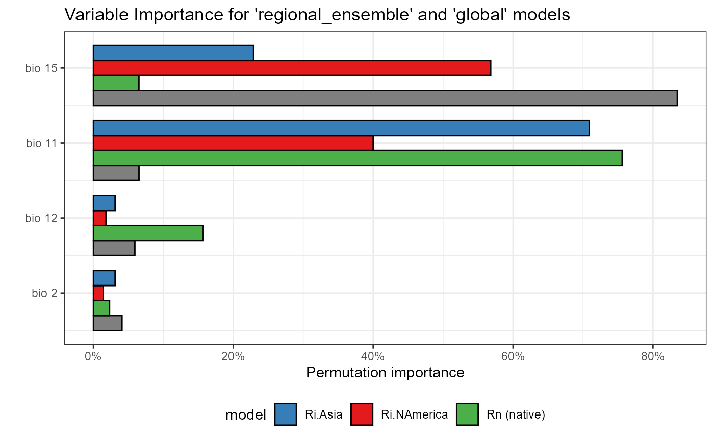
    title = "Variable Importance for 'regional_ensemble' and 'global' models",
    x = "",
    y = "Permutation importance"
    ) +
  scale_x_continuous(
    breaks = c(1, 2, 3, 4),
    labels = c("bio 2", "bio 12", "bio 11", "bio 15")
  ) +
  scale_y_continuous(labels = scales::percent) +
    # aes
  theme_bw() +
  scale_fill_manual(
    name = "model",
    values = ensemble_colors,
    aesthetics = "fill"
  ) +
  theme(legend.position = "bottom") +
  coord_flip()

var_imp_ensemble_global

ggsave(
  var_imp_ensemble_global, 
  filename = file.path(
    here::here(), "vignette-outputs", "figures", "Variable_importance_regional_ensemble_global.jpg"
    ),
  height = 8, 
  width = 8,
  device = jpeg,
  dpi = "retina"
  )