#1: Isolating dispersal jumps and diffusive spread
Nadege Belouard1
2024-08-22
Source:vignettes/010_Jump_list.Rmd
010_Jump_list.RmdAim and setup
The spread of invasive species is due both to diffusive spread and human-assisted jump dispersal, often caused by species hitchhiking on vehicles. The aim of this vignette is to differentiate diffusive spread from jump dispersal in invasive species based on occurrence data. This identification required the development of a directional analysis of species presence. We demonstrate this method using occurrence data of the spotted lanternfly, Lycorma delicatula, an invasive Hemiptera in the United States.
1. Data overlook
The SLF dataset is available from the lydemapr
companion package. In the download_data folder, then in
the v2_2023 subfolder, download the
lyde_data_v2.zip file and place it in the data
folder of your local jumpID project. At the date at which
this vignette is written, lydemapr contains data up to year
2022.
We load this dataset that contains all the occurrences of the spotted lanternfly, and take a look at it.
##   bio_year latitude longitude lyde_established
## 1     2015 40.41441 -75.65882            FALSE
## 2     2016 40.33333 -75.63529            FALSE
## 3     2016 40.36036 -75.48235            FALSE
## 4     2016 40.36937 -75.62353            FALSE
## 5     2016 40.37838 -75.71765            FALSE
## 6     2016 40.47748 -75.62353            FALSE
The dataset contains 831,039 rows, each corresponding to a SLF survey
at a specific date and location. The columns that we will using
are:
* bio_year: the biological year of the occurrence (see
lydemapr for a description of the difference between year
and bio_year)
* latitude and longitude (XY coordinates). The precise location of SLF
surveys is here summarized in 1-km² cells. All coordinates are in WGS84
(EPSG 4326)
* lyde_established: whether an established SLF population was found in
this survey (at least two live individuals or an egg mass, see
lydemapr)
2. Data formatting
First, to use the jumpID package, we need to rename the
columns with generic names expected by the package. We also remove rows
where the SLF establishment is NA.
slf %<>% rename(year = bio_year,
                established = lyde_established) %>%
  filter(is.na(established) == F)
Second, multiple surveys were sometimes conducted at the same location during the same year, resulting in a redundant dataset for the purpose of our analysis. We summarize the information available at each location every year, so that a row now represents the detection status at a location for a given year.
Note: when several surveys indicate that SLF are “present” the same year at the same location, it could be tempting to categorize SLF as “established”. However, the category “present” often refers to dead individuals, although this information is not explicitly available. We use a conservative approach and consider SLF as established in a cell only if one of the surveys considered it as established.
grid_data <- slf %>%
  dplyr::group_by(year, latitude, longitude) %>%
  dplyr::summarise(established = any(established)) %>%
  ungroup()
## `summarise()` has grouped output by 'year', 'latitude'. You can override using
## the `.groups` argument.
head(grid_data)## # A tibble: 6 × 4
## year latitude longitude established
## <int> <dbl> <dbl> <lgl>
## 1 2014 39.8 -76.8 FALSE
## 2 2014 39.8 -76.3 FALSE
## 3 2014 39.8 -76.4 FALSE
## 4 2014 39.9 -76.6 FALSE
## 5 2014 39.9 -76.9 FALSE
## 6 2014 39.9 -76.5 FALSEThe dataset now has 123,532 rows, corresponding to 1280 x 1596 cells. Let’s look at these data on a map.
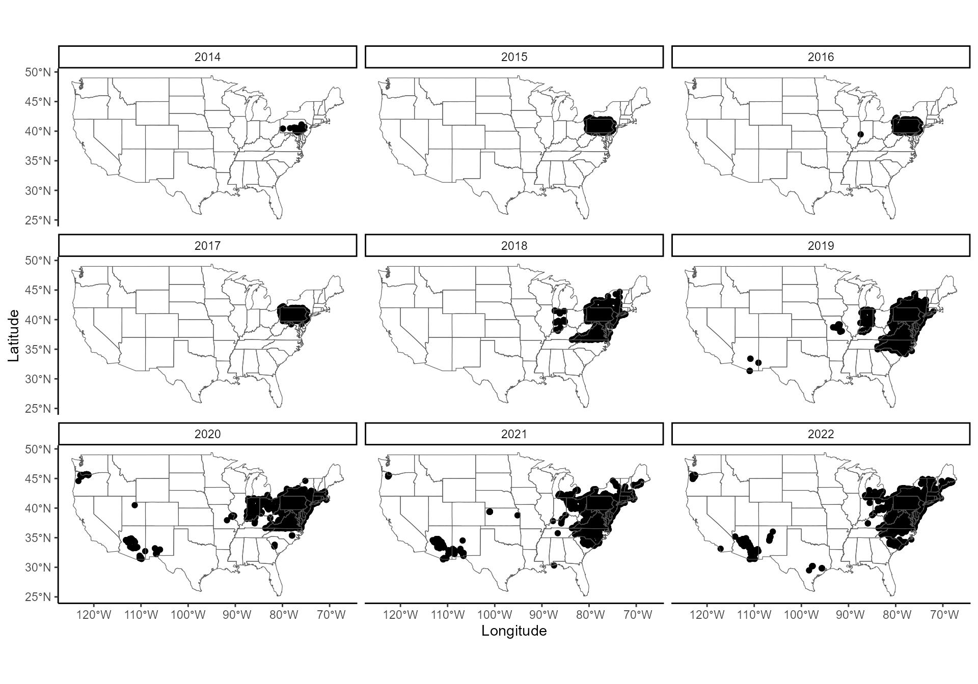
Cells were predominantly surveyed in the Eastern US, but there are also cells surveyed in other parts of the US, starting in 2019. Positive cells (established SLF) are only in the Eastern US, so maps will be zoomed in on the Eastern US from here.
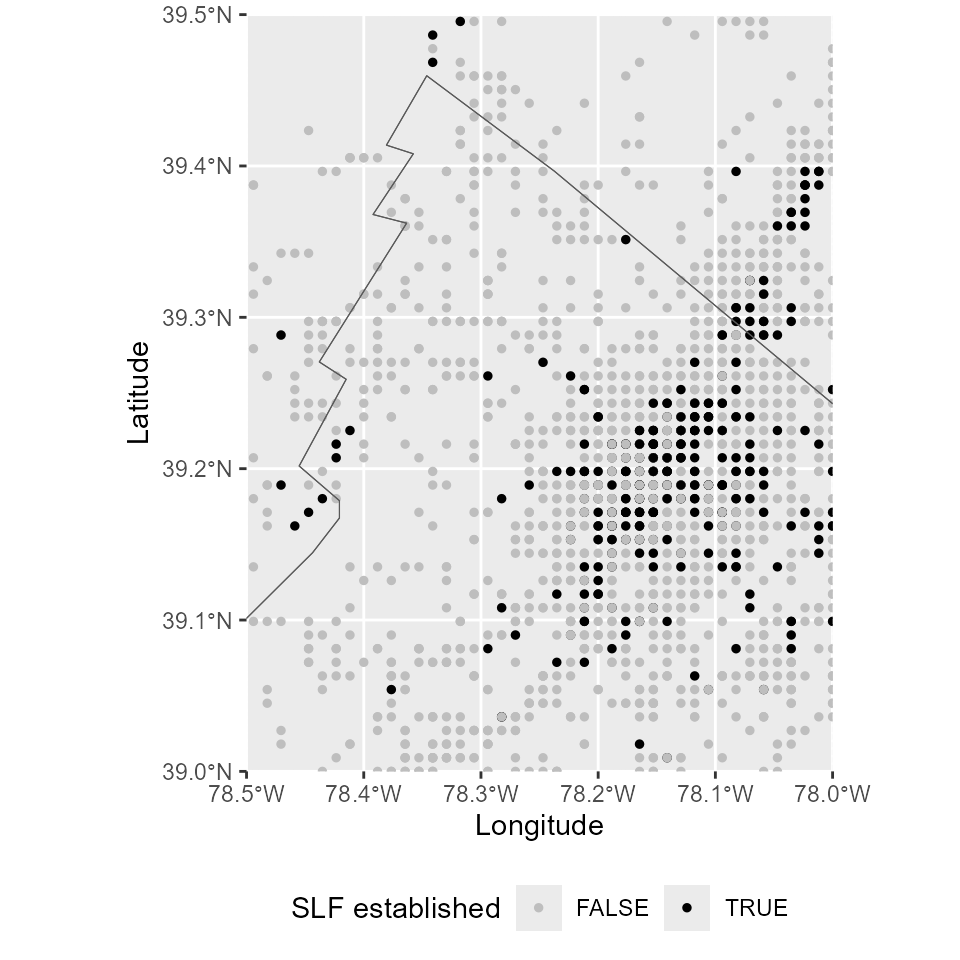
Every year, there is a large number of cells surveyed with positive (SLF established) or negative results (SLF not established). A zoomed-in map allows to see the cell grid.
The progression of the invasion will be measured starting from the introduction point that has been documented in Barringer et al. 2015. We store the coordinates of the introduction point in an object for the next analyses. If the precise introduction point is unknown, it may be replaced by the centroid of the invasion at the time the invasive species was discovered in the invasive range.
# Coordinates of the introduction site, extracted from Barringer et al. 2015
# As a table (for distance calculations):
centroid_df <- data.frame(longitude = -75.675340,
                        latitude = 40.415240)


# Replace by the centroid of the invasion in the first years of the invasion if the
# introduction point is unknown:
# centroid_df <- slf %>% filter(year == 2014) %>%
#   summarise(latitude = mean(.$latitude),
#             longitude = mean(.$longitude))
To finish preparing the dataset for analysis, we calculate the distance between each survey cell and the introduction point.
grid_data %<>%
  dplyr::mutate(DistToIntro = geosphere::distGeo(grid_data[,c('longitude','latitude')],
                                                 centroid_df[,c('longitude', 'latitude')])/1000)
# the distance is obtained in meters, and we divide it by 1000 to obtain kilometers
# given the scale of this invasion.

head(grid_data)
## # A tibble: 6 × 5
## year latitude longitude established DistToIntro
## <int> <dbl> <dbl> <lgl> <dbl>
## 1 2014 39.8 -76.8 FALSE 121.
## 2 2014 39.8 -76.3 FALSE 83.7
## 3 2014 39.8 -76.4 FALSE 90.4
## 4 2014 39.9 -76.6 FALSE 101.
## 5 2014 39.9 -76.9 FALSE 121.
## 6 2014 39.9 -76.5 FALSE 92.2The dataset is now ready for the jump analysis.
3. Differentiating diffusive spread and jump dispersal: principle
A set of four successive functions will be run to separate cells where SLF is established due to continuous, diffusive spread, from cells where SLF is established due to jump dispersal. We will first run the functions on a tentative set of parameters to understand how the analysis works. The optimization of the parameters will be described later in this vignette.
a- attribute_sectors()
Considering that the expansion of the invasion is heterogeneous in
space, the jump analyses requires the invasion range to be divided into
sectors with the introduction site as the origin. The first function,
attribute_sectors() attributes a sector number to each cell
of the dataset, to be used in the jump analysis. Here, we divide the
invasion range into 16 sectors. See vignette #2 “Decreasing calculation
time” to learn how changing the number of sectors may make your analysis
faster.
grid_data_sectors <- jumpID::attribute_sectors(dataset = grid_data,
                                                 # dataset to be explored
                             nb_sectors = 16,
                             # number of sectors to divide the invasion range
                             centroid = c(-75.675340, 40.415240)
                             # vector containing the centroid coordinates as long/lat
                             )
## 2024-08-22 14:34:47.474122 Start sector attribution... Sector attribution completed.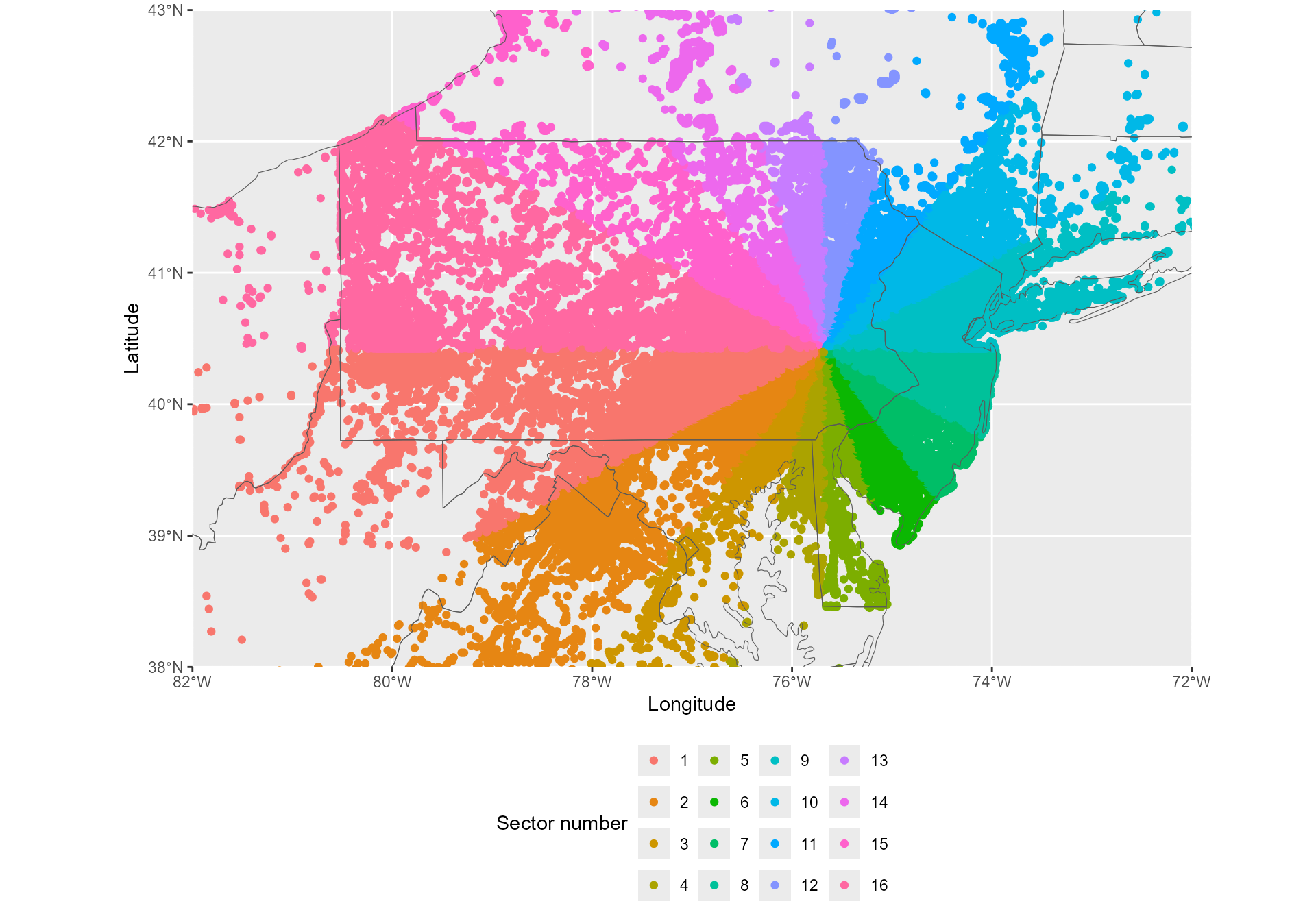
The jump analysis will go through each sector successively.
b- find_thresholds()
The function find_thresholds() will then search for the
first discontinuity in the SLF distribution. Points are sorted by
increasing distance to the introduction point, and the function goes
through each consecutive pair of points, starting from the introduction
point and going outwards. It stops once it identifies a distance larger
than a defined gap_size between two consecutive points,
marking a discontinuity in the SLF distribution. The last point before
this discontinuity marks the putative limit of the diffusive spread. The
function runs independently for each sector. It is considered that
populations do not go extinct, and data are cumulated over time. The
limit of diffusive spread cannot go back towards the introduction point
over time.
The input dataset is the output of attribute_sectors(). The
gap_size parameter defines the minimal distance between two
consecutive points that marks a discontinuity in the SLF distribution,
in km. In this example, it is set to 15 km.
If the option “negatives” is set to TRUE (default), the function will
check that there are negative surveys in the discontinuity, so that the
absence of SLF established is not due to an absence of surveys in the
area.
gap_size = 15

Results_thresholds <- jumpID::find_thresholds(dataset = grid_data_sectors,
                                                gap_size = gap_size,
                                                negatives = T)
## 2024-08-22 14:35:00.539064 Start finding thresholds... Sector 1/16... 2/16... 3/16... 4/16... 5/16... 6/16... 7/16... 8/16... 9/16... 10/16... 11/16... 12/16... 13/16... 14/16... 15/16... 16/16
## Threshold analysis done. 4243 potential jumps were found.
# Resulting objects are
#- Results_thresholds$preDist, a data frame of threshold cells = extreme points of the
# diffusive spread. Will be completed in find_secDiff()
#- Results_thresholds$potJumps, a data frame of potential jumps. Will be
# pruned in find_jumps()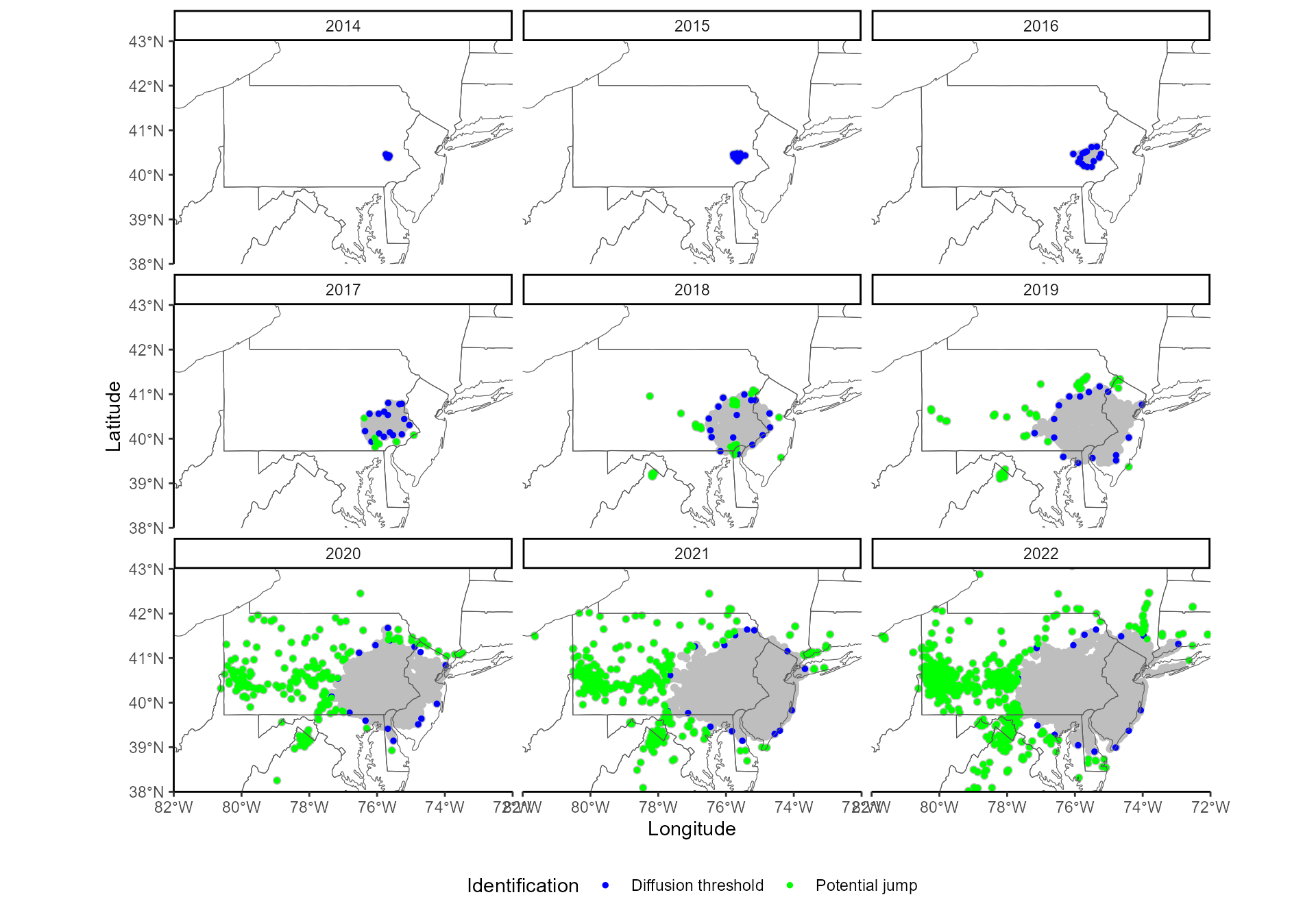
On this map, blue points indicate the invasion front identified by
find_thresholds(), i.e., the limits of the diffusive spread
in every direction, for every year. At this point of the analysis, all
points farther than these thresholds are stored as potential jumps
(green points).
c- find_jumps()
The function find_jumps() prunes the list of potential
jumps of cells that are less than Jumps.
Results_jumps <- jumpID::find_jumps(grid_data = grid_data,
                       potJumps = Results_thresholds$potJumps,
                       gap_size = gap_size)
## 2024-08-22 14:41:08.43217 Start finding jumps... Year 2014 ... Year 2015 ... Year 2016 ... Year 2017 ... Year 2018 ... Year 2019 ... Year 2020 ... Year 2021 ... Year 2022 ... Jump analysis done. 387 jumps were identified.
# Resulting objects are:
#- Results_jumps$Jumps, a data frame containing all jumps
#- Results_jumps$diffusers, a data frame of positive cells stemming from diffusive spread
#- Results_jumps$potDiffusion, a data frame of remaining cells, containing a mix of
# secondary diffusion and additional threshold points. Will be pruned in find_secDiff()
The analysis may be stopped here if only dispersal jumps are of
biological interest. As a complement, secondary diffusion may be
examined in the last function, find_secDiff().
d- find_secDiff()
Cells that were discarded from the jump list are either additional
threshold points or secondary diffusion from a previous jump.
find_secDiff() attributes them to the correct category by
checking whether they are close from a previous jump, or a diffusion
point.
Results_secDiff <- jumpID::find_secDiff(potDiffusion = Results_jumps$potDiffusion,
                                Jumps = Results_jumps$Jumps,
                                diffusers = Results_jumps$diffusers,
                                Dist = Results_thresholds$preDist,
                                gap_size = gap_size)
## 2024-08-22 14:41:53.572058 Start finding secondary diffusion... Year 2017 ...Year 2018 ...Year 2019 ...Year 2020 ...Year 2021 ...Year 2022 ...Analysis of secondary diffusion done.
# Resulting objects are:
#- Results_secDiff$secDiff, a data frame of all cells that are secondary diffusion
# from a previous jump
#- Results_secDiff$Dist, a data frame of all extreme points on the invasion front (thresholds)
4. Wrapper for jump analysis
All these analyses can be done in one instance using the wrapper function.
jumps_wrapper <- jumpID::find_jumps_wrapper(dataset = grid_data,
                                              nb_sectors = 16,
                                              centroid = c(-75.675340, 40.415240),
                                              gap_size = 15,
                                              negatives = T)
## 2024-08-22 14:43:16.131378 Start sector attribution... Sector attribution completed.
## 2024-08-22 14:43:16.164782 Start finding thresholds... Sector 1/16... 2/16... 3/16... 4/16... 5/16... 6/16... 7/16... 8/16... 9/16... 10/16... 11/16... 12/16... 13/16... 14/16... 15/16... 16/16
## Threshold analysis done. 4243 potential jumps were found.
## 2024-08-22 14:49:13.378279 Start finding jumps... Year 2014 ... Year 2015 ... Year 2016 ... Year 2017 ... Year 2018 ... Year 2019 ... Year 2020 ... Year 2021 ... Year 2022 ... Jump analysis done. 387 jumps were identified.
## 2024-08-22 14:49:39.405896 Start finding secondary diffusion... Year 2017 ...Year 2018 ...Year 2019 ...Year 2020 ...Year 2021 ...Year 2022 ...Analysis of secondary diffusion done.We plot the results on a map.
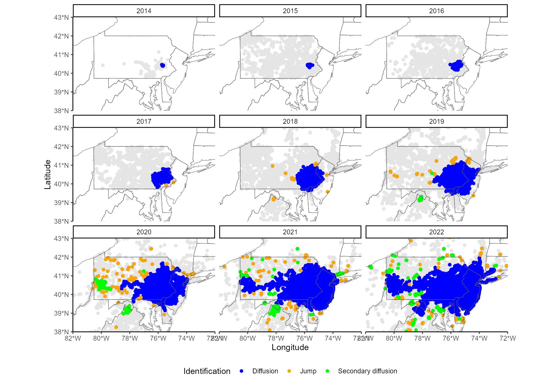
5. Rarefy jump clusters
Some jumps were clustered in the same area. Jump clusters may stem from independent dispersal jumps, i.e. SLF hitchhiked multiple times to these locations the same year. Alternatively, jump clusters may result from SLF quickly spreading around a single dispersal jump. Finally, they can be a mix between these two hypotheses. We identify these jump clusters to better understand jump locations.
First, we delineate these jump clusters as jumps located less than the gap size from each other. Check how many points there are per jump cluster.
a- group_jumps()
Jump_groups <- jumpID::group_jumps(Jumps, gap_size = 15)## `summarise()` has grouped output by 'year'. You can override using the
## `.groups` argument.
## `summarise()` has grouped output by 'year'. You can override using the
## `.groups` argument.## # A tibble: 6 × 2
## year mean_njumps
## <int> <dbl>
## 1 2017 1.5
## 2 2018 8.29
## 3 2019 4.23
## 4 2020 1.65
## 5 2021 2.28
## 6 2022 2.41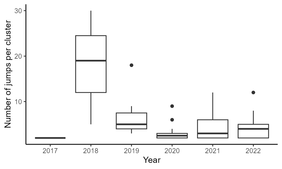
b- rarefy_groups()
We summarize each jump cluster by summarizing each of them by their most central point.
Jump_clusters <- jumpID::rarefy_groups(Jump_groups) %>%
  dplyr::mutate(Rarefied = TRUE)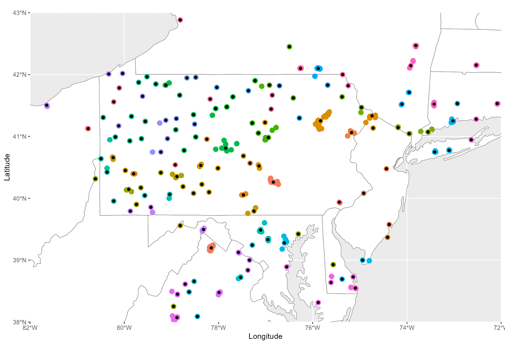
These 387 jumps were rarefied into 152 jump
clusters.