#1B Creating the figures associated with the jump analysis
Nadege Belouard1
Isabella G. Smith2
2024-08-22
Source:vignettes/011_Figures_jump_list.Rmd
011_Figures_jump_list.RmdAim and setup
This vignette computes all the figures included in the manuscript
that is associated with the jumpID package. This vignette
requires loading data frames generated in the first vignette of this
package.
Load files generated in the previous vignette
slf <- read.csv(file.path(here::here(), "data", "lyde_data_v2", "lyde.csv"), h=T)
grid_data <- read.csv(file.path(here::here(), "exported-data", "grid_data.csv"), h=T)
centroid <- data.frame(longitude_rounded = -75.675340, latitude_rounded = 40.415240)
Jumps <- read.csv(file.path(here::here(), "exported-data", "jumps.csv"))
Jump_clusters <- read.csv(file.path(here::here(), "exported-data", "jump_clusters.csv"))
Thresholds <- read.csv(file.path(here::here(), "exported-data", "thresholds.csv"))
diffusion <- read.csv(file.path(here::here(), "exported-data", "diffusion.csv"))
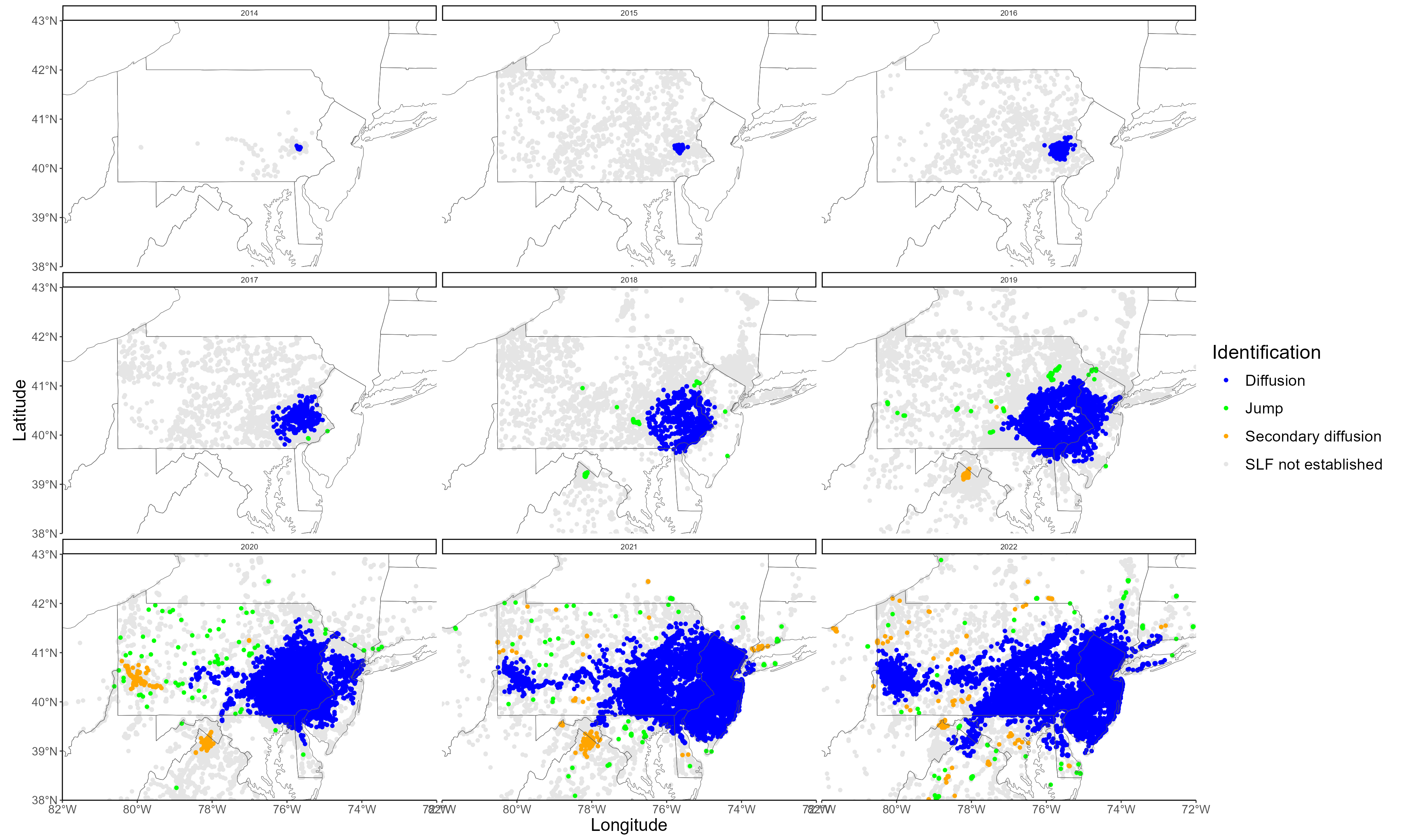
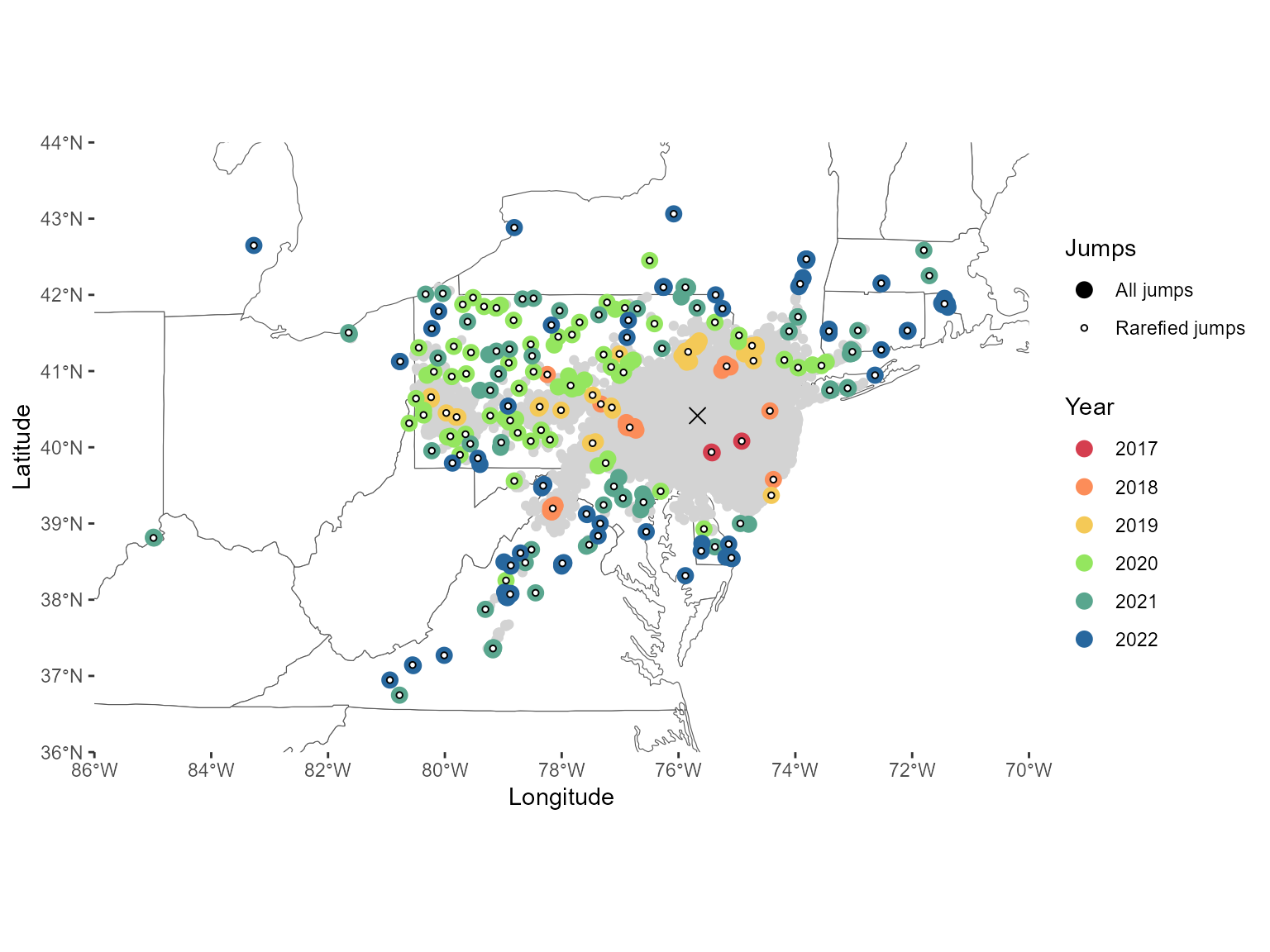
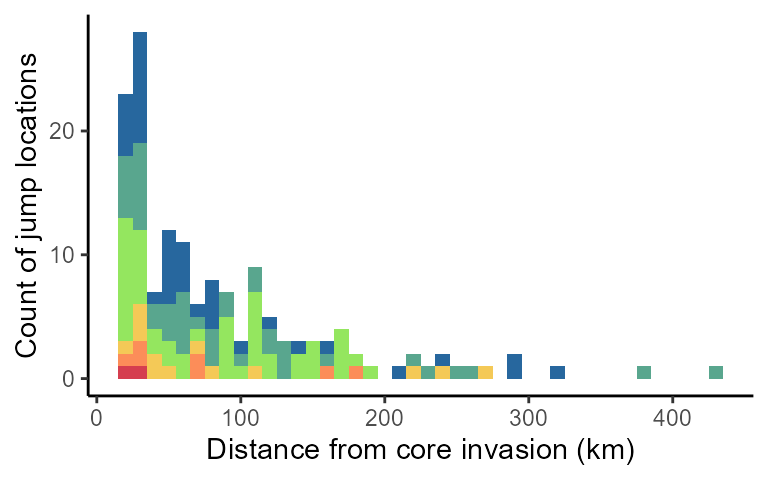
secDiffusion <- read.csv(here::here("exported-data", "secdiffusion.csv"))Figure 2: Faceted jump map, barplot & distance

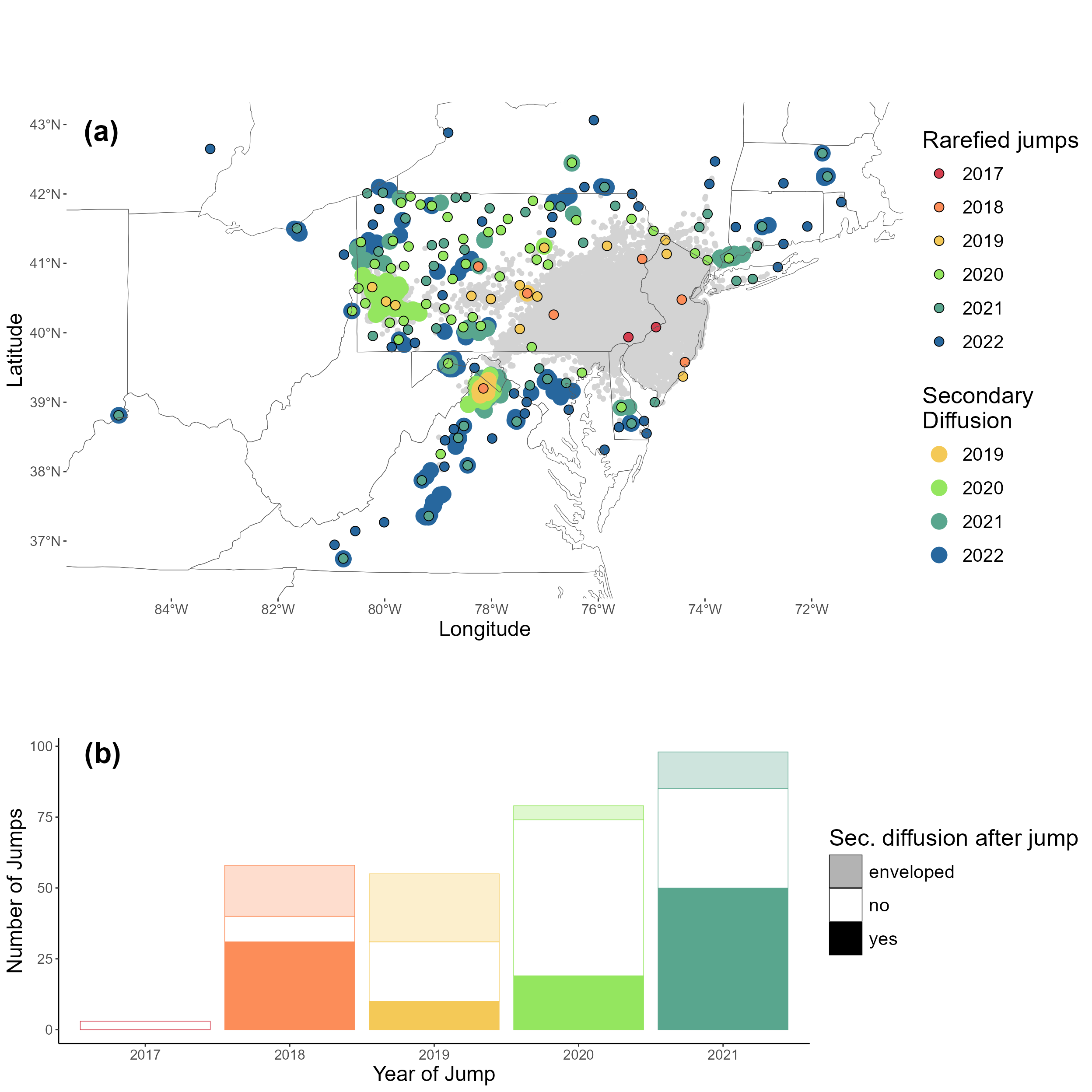
2C: distance of jumps box plot
calculate the distance between the invasion front and jumps every year
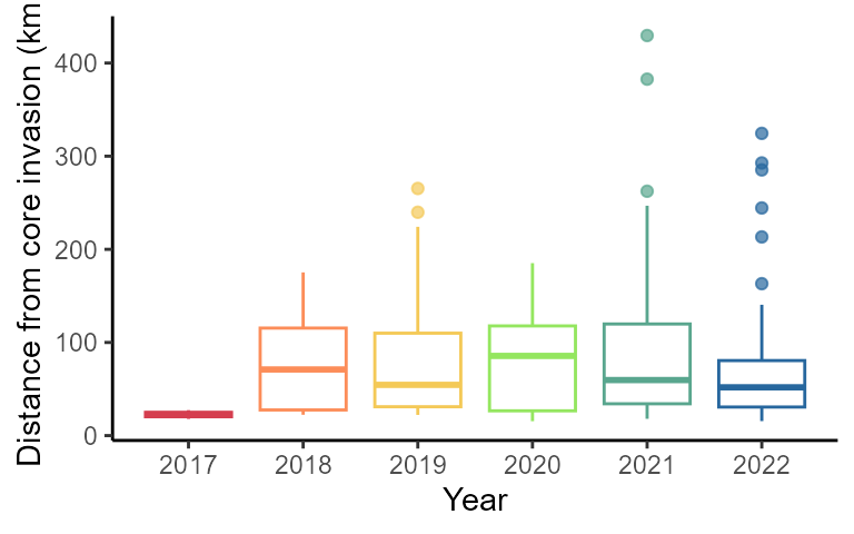
2D Evolution of jump distances
Linear model for statistical test
# generate model
model <- lm(log(DistToFront) ~ year, data = Jump_clusters)
# look at residuals
hist(model$residuals)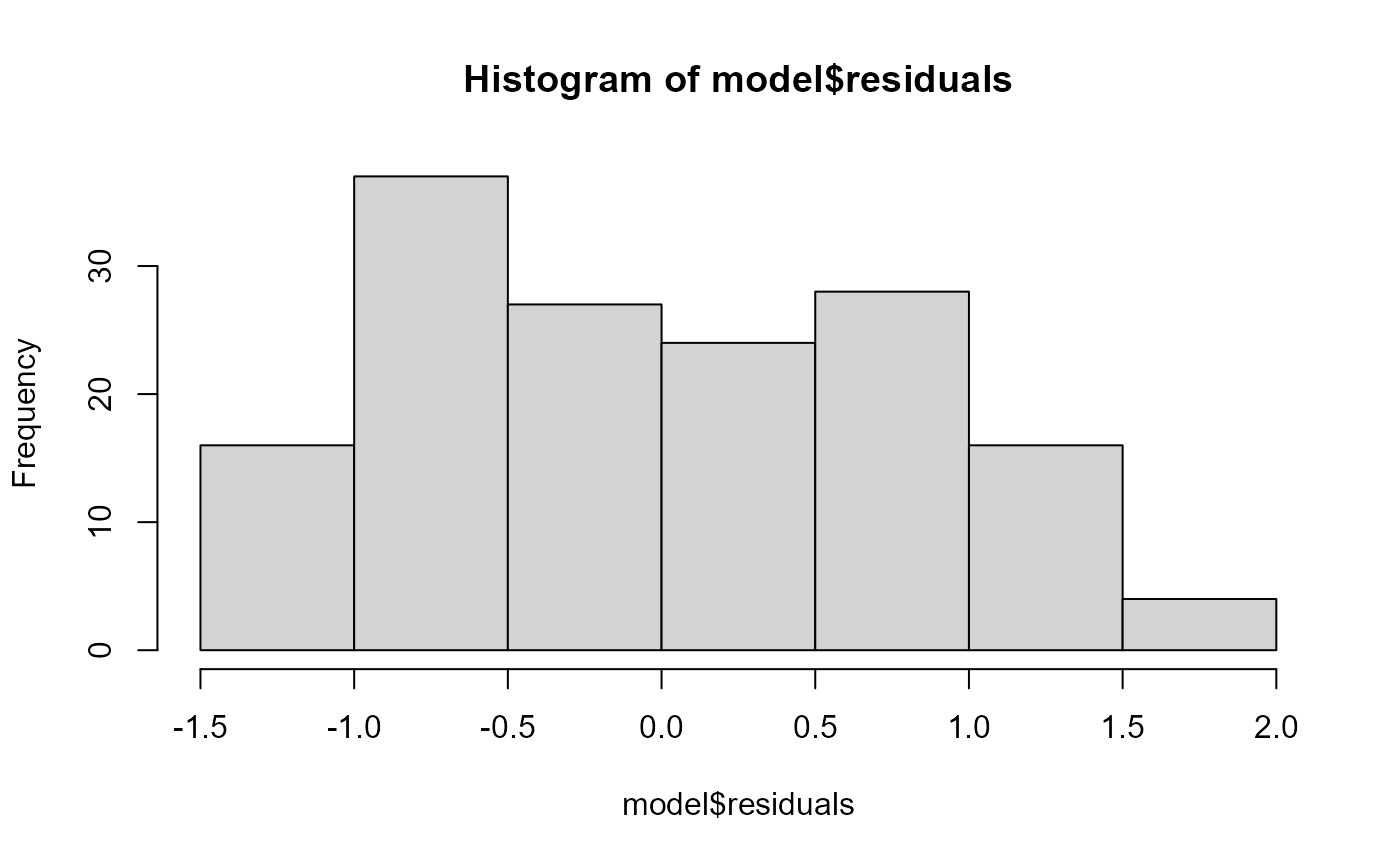
# look at results
summary(model)
##
## Call:
## lm(formula = log(DistToFront) ~ year, data = Jump_clusters)
##
## Residuals:
## Min 1Q Median 3Q Max
## -1.41134 -0.74153 -0.09242 0.61409 1.92588
##
## Coefficients:
## Estimate Std. Error t value Pr(>|t|)
## (Intercept) -38.04036 115.38662 -0.330 0.742
## year 0.02087 0.05711 0.365 0.715
##
## Residual standard error: 0.8217 on 150 degrees of freedom
## Multiple R-squared: 0.0008896, Adjusted R-squared: -0.005771
## F-statistic: 0.1336 on 1 and 150 DF, p-value: 0.7153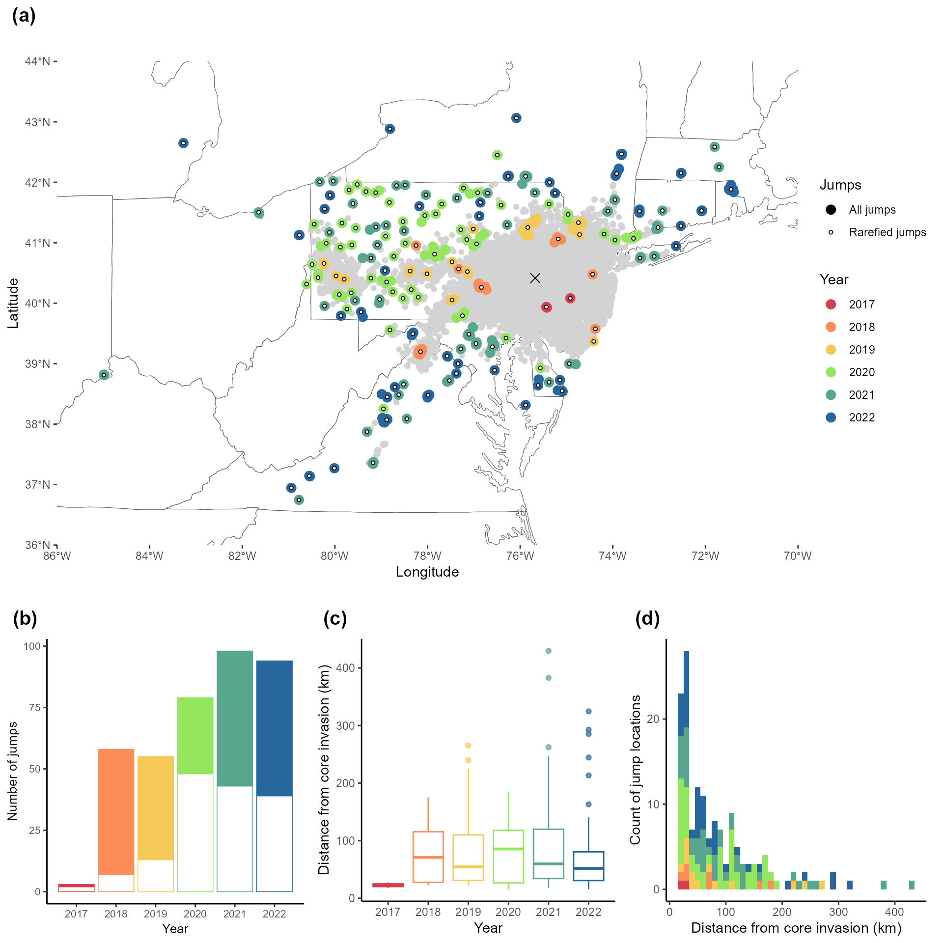
Figure 3: Invasion radius
To estimate the spread of the SLF, we extract for each year the radius of the invasion in each sector. We can look at how the radius of the invasion increases over time, when differentiating diffusive spread and jump dispersal.
Test the difference in invasion radius between spread types
# generate model
model <- lm(log(maxDistToIntro) ~ year*Type, data = radiusData)
# look at residuals
hist(model$residuals, breaks = 30)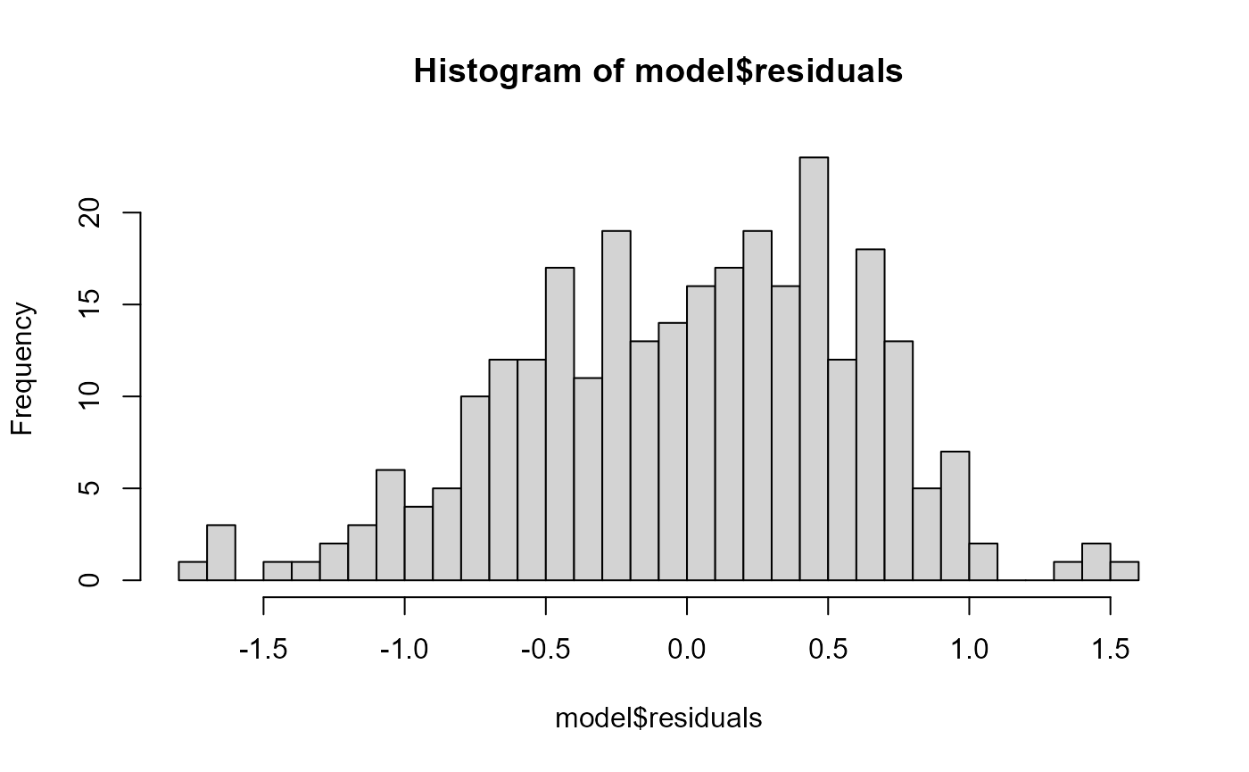
# look at results
anova(model)
## Analysis of Variance Table
##
## Response: log(maxDistToIntro)
## Df Sum Sq Mean Sq F value Pr(>F)
## year 1 552.44 552.44 1510.4347 < 2.2e-16 ***
## Type 1 2.92 2.92 7.9834 0.005058 **
## year:Type 1 1.89 1.89 5.1753 0.023661 *
## Residuals 282 103.14 0.37
## ---
## Signif. codes: 0 '***' 0.001 '**' 0.01 '*' 0.05 '.' 0.1 ' ' 1Calculate the yearly increase in invasion radius
# All spread:
meanRadius %>% filter(Type == "All spread") %>%
  mutate(radiusIncrease = c(NA, diff(mean))) %>%
  summarise(mean = mean(radiusIncrease, na.rm = T),
            sd = sd(radiusIncrease, na.rm = T))
## # A tibble: 1 × 2
## mean sd
## <dbl> <dbl>
## 1 41.3 23.6
# Invasion front:
meanRadius %>% filter(Type == "Invasion front") %>%
  mutate(radiusIncrease = c(NA, diff(mean))) %>%
  summarise(mean = mean(radiusIncrease, na.rm=T),
            sd = sd(radiusIncrease, na.rm = T))
## # A tibble: 1 × 2
## mean sd
## <dbl> <dbl>
## 1 25.1 11.4