Aim and Scope
Here we calculate the geographic, landscape, and economic attributes for island banks in the Caribbean Bioregion as delineated by Hedges et al. (2019) and including Bermuda.
First we need to load in the caribmacro package.
# Project package
library(caribmacro)
If you do not have this package installed, then run
devtools::load_all in order to load all of the necessary
functions if you are running this code in the caribmacro R project in
the shared folder. If you are not, then see the functions vignette for
the Functions needed.
# Load all of the functions of the caribmacro package
devtools::load_all("./", export_all = FALSE)

## Function needed ##
#   'isolation'  -> calculates the isolation metric(s)
#   'factorize'  -> turns character columns of a data frame into factors
The other R packages needed for this are:
Bank Attributes
Bank Geography
In order to determine the island bank (hereafter, bank) land area, number of islands, and island spread, we need to load in the Caribbean island and bank shapefiles from the ‘data_raw’ folder in the ‘caribmacro’ package.
# loading data
carib.isl <- st_read(file.path(here(), 'data_raw', 'gis', 'Carib_Islands.shp'))
carib.bnk <- st_read(file.path(here(), 'data_raw', 'gis', 'Carib_Banks.shp'))
The in order to be able to calculate the bank area, we need to re-project the shapefiles into the Lambert Azimuthal Equal Area projection centered in the Caribbean. Then, we must change the type of object to a spatial object.
# Re-project into Lambert Azimuthal Equal Area centered in the Caribbean
carib.isl <- st_transform(carib.isl, "+proj=laea +x_0=0 +y_0=0 +lon_0=-72 +lat_0=20")
carib.bnk <- st_transform(carib.bnk, "+proj=laea +x_0=0 +y_0=0 +lon_0=-72 +lat_0=20")

# Change 'carib.isl' and 'carib.bnk' to class 'Spatial'
carib.isl <- as(carib.isl, Class = "Spatial")
carib.bnk <- as(carib.bnk, Class = "Spatial")
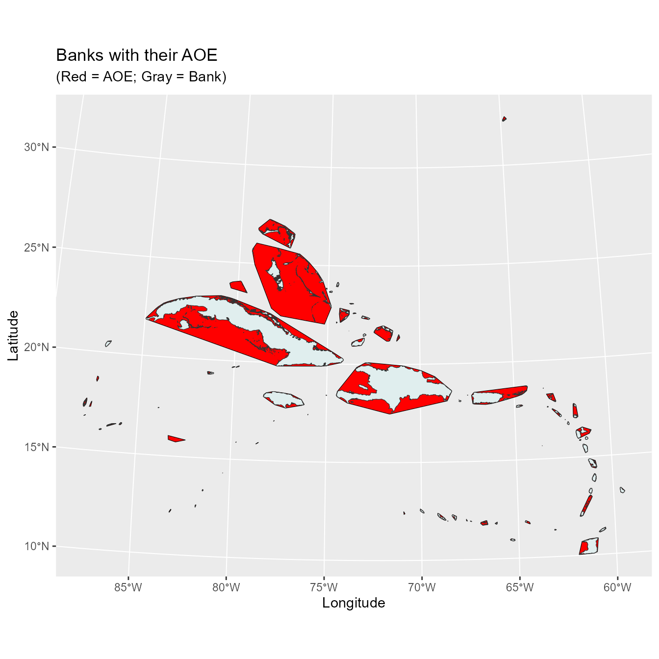
Before we calculate the land area of each bank lets create a maximum convex polygon (MCP) around each bank in order to calculate the spread of each bank’s islands.
bnk.mcp <- gConvexHull(carib.bnk, byid = TRUE)

bnk.mcp.sf <- st_as_sf(bnk.mcp)
bnk.mcp.sf$bank <- st_as_sf(carib.bnk)$bank
Let’s now take a look at these MCPs to see if they look appropriate.
Now we calculate the bank area using the Islands shapefile.
carib.isl.sf <- st_as_sf(carib.isl)
isl.area <- data.frame(bank = carib.isl.sf$bank, Area = as.numeric(st_area(carib.isl.sf)))

bnk.area <- aggregate(Area ~ bank, data = isl.area, sum)
With the bank area we then determine the area of the MCPs (i.e. area of extent, hereafter AOE) and use that to calculate the island spread of each bank by dividing the bank area by the AOE and subtracting that from one. We also will determine the number of islands in each bank and combine all of this into one data frame, ‘X’.
X <- data.frame(bank = bnk.mcp.sf$bank, AOE = as.numeric(st_area(bnk.mcp.sf)))

X <- merge(bnk.area, X, by='bank', all=TRUE)

X$Area <- X$Area/1000000 #divide by 1E6 to convert to km^2
X$AOE <- X$AOE/1000000   #divide by 1E6 to convert to km^2

X$Spread <- 1 - (X$Area/X$AOE) #'1 - ' so large values = more spread

isl.area$Number <- 1
X <- merge(X, aggregate(Number ~ bank, data = isl.area, sum), by='bank', all=TRUE)
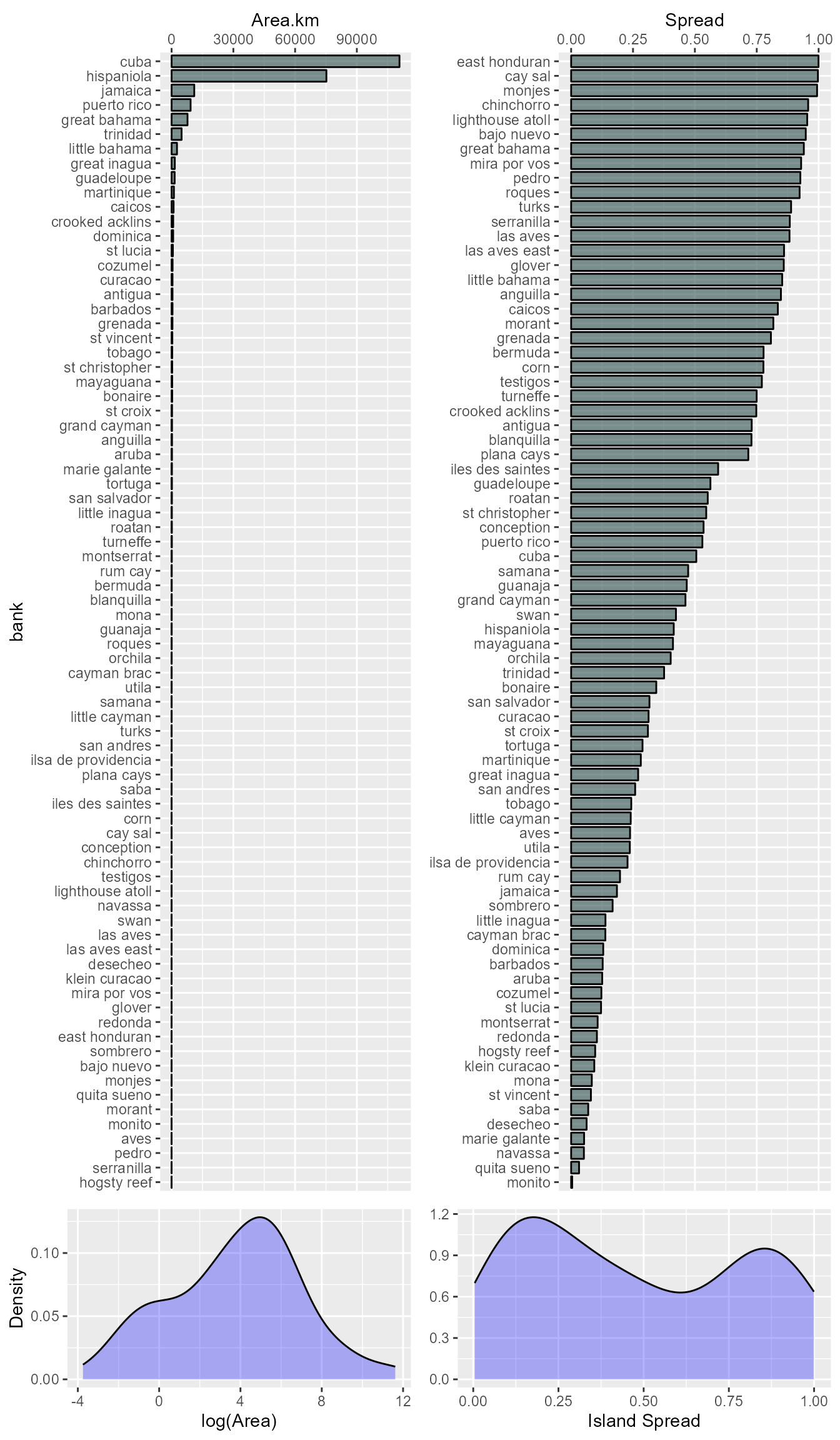
Now let’s look at the distribution of the bank area and island spread variables.
Bank Landcover and Elevation
Now let’s start to incorporate other bank attributes into the bank data for use in the analysis. Let’s start by loading in the bank elevation and land cover data. This data was exported from Google Earth Engine using the ecoEE module (Helmus et al 2020; JavaScript scripts can be found at the project GitHub page or within the Earth Engine vignette). The bank elevation data was extracted from a SRTM digital elevation model (http://srtm.csi.cgiar.org), and the land cover data was extracted from the MODIS Land Cover Type Yearly Global 500m data set (DOI: 10.5067/MODIS/MCD12Q1.006) using the Annual International Geosphere-Biosphere Programme (IGBP) classification. We then combine the elevation data with the previously calculated bank geographic data, and the land cover data to create a new ‘lndcvr’ data frame.
For the land cover we combine the “Cropland” and “Urban” values to get percent anthropogenic land cover. Similarly, we combine “Evr_Needle”, “Grassland”, “Wetland”, “Evr_Broad”, “Dec_Needle”, “Dec_Broad”, “Mixed_For”, “C_Shrub”, “O_Shrub”, “W_Savanna”, and “Savanna” to get percent green land cover (i.e. ‘natural’). Additionally, pixels that were made up of mosaics of small-scale cultivation 40-60% with natural tree, shrub, or herbaceous vegetation were given the classification as “Crp_Nat”, half of which was added to percent green cover and half added to anthropogenic land cover.
For small banks, the pixels may have been determined as permanent wetland when they were actually urban due to the small area of the landmass (i.e. the ocean made the pixel permanently inundated with 30-60% water cover). Because of this, we “ground-truthed” the data for the smaller banks (\(\leq\) 100km2) by looking at the most recent Google Earth images of the bank and comparing with the raster data to see if pixels erroneously determined as permanent wetland. If the pixel had mostly buildings in it then the pixel was added to “Urban” and removed from “Wetland”. An example of this is Bermuda which is considered almost entirely permanent wetland when in fact most of the land area has urban development.
# Bank Elevation
elev <- read.csv(file.path(here(), 'data_raw', 'IBT_Bank_Elevation_final.csv'), header = TRUE)
names(elev)[which(names(elev) != 'bank')] <- paste('DEM', names(elev)[which(names(elev) != 'bank')], sep = '.')

X <- merge(X, elev[, c('bank', 'DEM.max', 'DEM.mean', 'DEM.sd')], by = 'bank', all = TRUE)
X <- X[order(X$bank), ]

# Bank land cover
igb_lc <- read.csv(file.path(here(), 'data_raw', 'IBT_Landcover_IGBP_final.csv'), header = TRUE)

igb_lc$anthro <- rowSums(igb_lc[, c("Cropland", "Urban")])
igb_lc$anthro <- (0.5 * igb_lc[, "Crp_Nat"]) + igb_lc$anthro

igb_lc$green <- rowSums(igb_lc[, c("Evr_Needle", "Grassland", 'Wetland', "Evr_Broad", "Dec_Needle",
                                    "Dec_Broad", "Mixed_For", "C_Shrub", "O_Shrub",
                                    "W_Savanna", "Savanna")])
igb_lc$green <- (0.5 * igb_lc[, "Crp_Nat"]) + igb_lc$green

lndcvr <- igb_lc[, c('bank', 'anthro', 'green')]
lndcvr <- lndcvr[order(lndcvr$bank), ]
Let’s look at the distribution of the land cover variables as well.
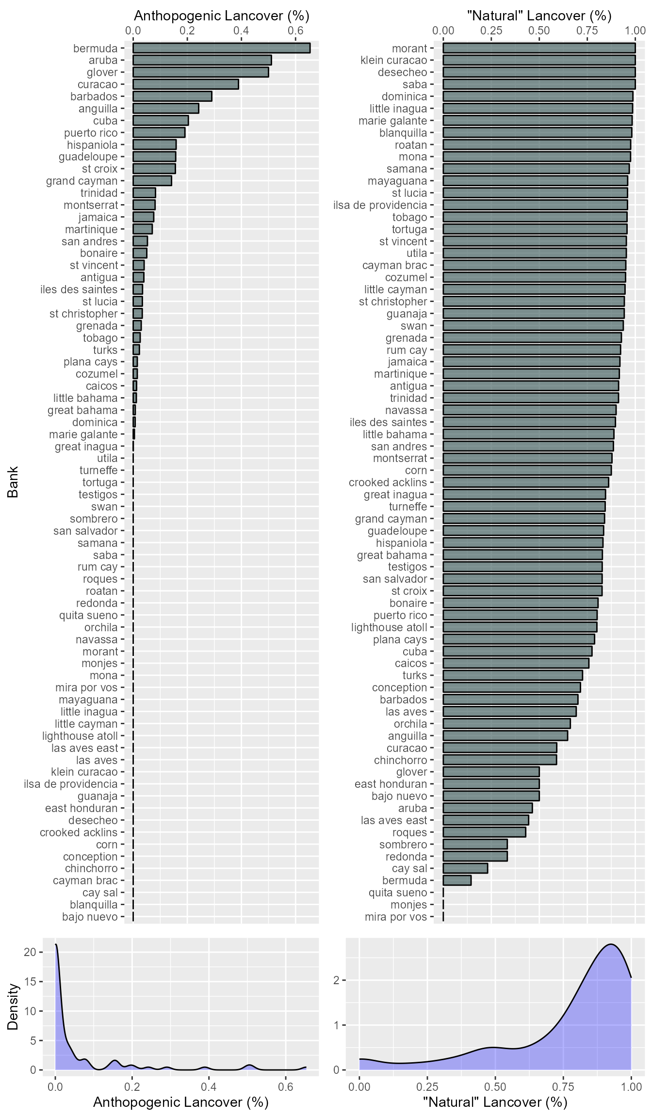
## Banks with no land cover data:
##  aves | hogsty reef | monito | pedro | serranilla
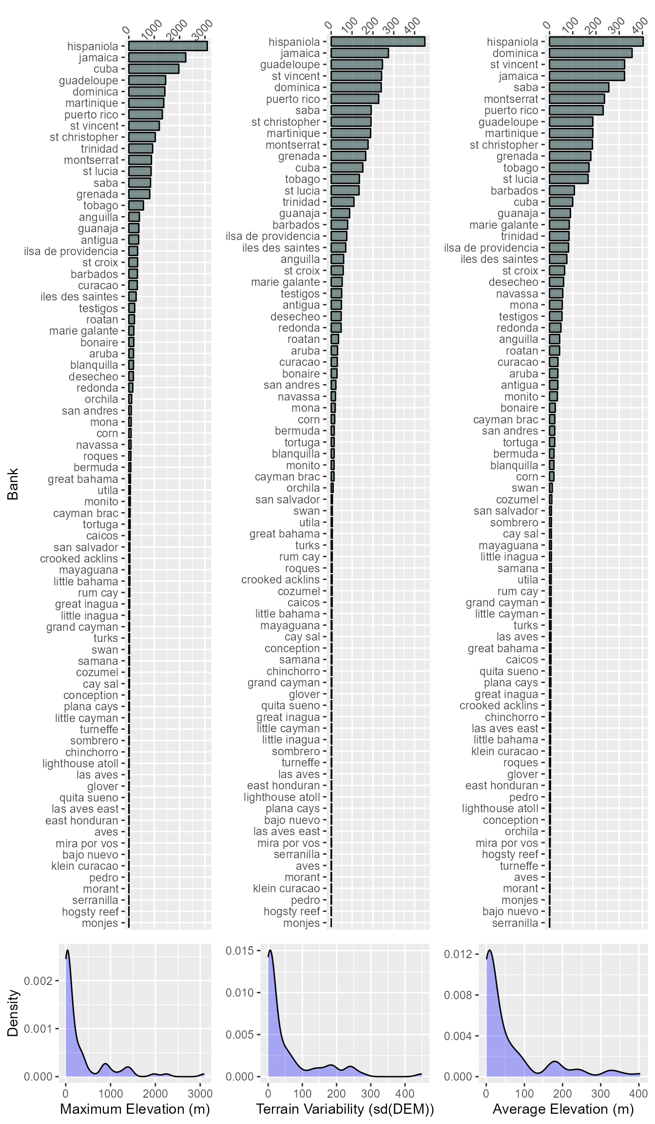
We also should look at the distribution on the various elevation distributions.
Bank Isolation
Bank isolation was calculated in a similar way as Helmus (2014) (DOI: 10.1038/nature13739). For this we will use the distances from the centroids of each bank, and then using that distance matrix calculate the isolation metrics by determining the principle components from a principle components anlysis (PCA) of selected square-root transformed distances to to other banks and source(s).
For the distances between the banks we will be using the bank centroids, so let’s load in the centroids and take a look at there placement.
cent <- st_read(file.path(here(), 'data_raw', 'gis', 'Centroids_Bank_Main.shp'))
map <- st_read(file.path(here(), 'data_raw', 'gis', 'Carib_Banks_w_Mainland.shp'))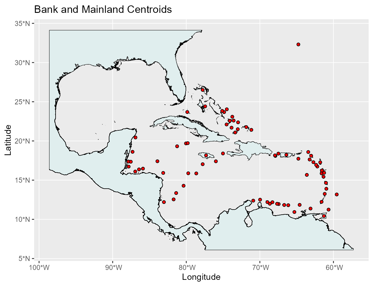
The placement of the centroids look good so now lets calculate the distance matrix that will hold all of the distances between the banks.
cent <- st_transform(cent, "+proj=aeqd +x_0=0 +y_0=0 +lon_0=-72 +lat_0=20")

cent.dist <- st_distance(x = cent, y = cent, by_element = FALSE)

cent.dist <- data.frame(cent.dist)
names(cent.dist) <- gsub(' ', '.', cent$bank)
cent.dist$bank <- cent$bank
row.names(cent.dist) <- gsub(' ', '.', cent.dist$bank)
cent.dist <- cent.dist[order(cent.dist$bank), c('bank', sort(names(cent.dist)[which(names(cent.dist) != 'bank')]))]

for (i in 2:ncol(cent.dist)) {
  cent.dist[, i] <- as.numeric(cent.dist[, i])
}
However, it makes more sense to use the shoreline of the mainland instead of centroids. That would ensure that island banks such as Trinidad are not considered isolated from the mainland even though it’s centroid is one of the closest to the South American shoreline. To do this we will have to load in another shapefile with the shorelines of North America, Central America, and South America and find the distance from all of the bank centroids to the the shoreline of the mainland. Those distances then need to be merged with the centroid distance matrix made above and the distance to the mainland centroids removed.
# Load the shapefile for the mainland shoreline
main.shor<-st_read(file.path(here(), 'data_raw', 'gis', 'Cont_Main_WGS_Merc.shp'))
main.shor <- st_transform(main.shor, "+proj=aeqd +x_0=0 +y_0=0 +lon_0=-72 +lat_0=20")
dist.shor <- st_distance(x = cent, y = main.shor, by_element = FALSE)

dist.shor <- data.frame(dist.shor)
names(dist.shor) <- gsub(' ', '.', main.shor$Isl_Name)
dist.shor$bank <- cent$bank
dist.shor <- dist.shor[order(dist.shor$bank), c('bank', sort(names(dist.shor)[which(names(dist.shor) != 'bank')]))]

for (i in 2:ncol(dist.shor)) {
  dist.shor[, i] <- as.numeric(dist.shor[, i])
}

dist.shor <- merge(cent.dist, dist.shor, by = 'bank', all = TRUE)
names(dist.shor) <- gsub('.y', '', names(dist.shor), fixed = TRUE)
shor.dist <- dist.shor[, intersect(names(cent.dist), names(dist.shor))]
For the Caribbean herpetofauna, South America was the main source for the immigration of species to the islands. However, work done with Anolis lizards has shown that many of the Anolis communities of the southern Greater Antilles and northern Lesser Antilles actually came from Cuba and Hispanola. Both of these banks are quite large being almost an order of magnitude greater in size than the next largest bank and seemed to have acted as a source for many of the surrounding islands. Therefore, in the same manner as the mainland, it makes sense to measure distance to these banks as distance to the shoreline of their main islands instead of their centroids.
# Load the shapefile for the Cuba and Hispaniola shoreline
sorc.shor<-st_read(file.path(here(), 'data_raw', 'gis', 'Cuba_Hisp_Shore.shp'))
sorc.shor <- st_transform(sorc.shor, "+proj=aeqd +x_0=0 +y_0=0 +lon_0=-72 +lat_0=20")
dist.sorc <- st_distance(x = cent, y = sorc.shor, by_element = FALSE)

dist.sorc <- data.frame(dist.sorc)
names(dist.sorc) <- gsub(' ', '.', sorc.shor$bank)
dist.sorc$bank <- cent$bank
dist.sorc <- dist.sorc[order(dist.sorc$bank), c('bank', sort(names(dist.sorc)[which(names(dist.sorc) != 'bank')]))]

for (i in 2:ncol(dist.sorc)) {
  dist.sorc[, i] <- as.numeric(dist.sorc[, i])
}

dist.sorc <- merge(shor.dist, dist.sorc, by = 'bank', all = TRUE)
names(dist.sorc) <- gsub('.y', '', names(dist.sorc), fixed = TRUE)
sorc.dist <- dist.sorc[, intersect(names(cent.dist), names(dist.sorc))]

row.names(sorc.dist) <- gsub(' ', '.', sorc.dist$bank)
dist <- sorc.dist[, names(sorc.dist)[which(names(sorc.dist) != 'bank')]]
Now that we have the distances between each bank and the distances
between the banks and the mainland, we can calculate the isolation
metrics. We will do this by using the isolation() function
in the ‘caribmacro’ package which calculates the isolation metrics in
the manner described above. For the calculation of island bank isolation
we will be using the square root transformed minimum distance to an
immigration source (Cuba, Hispaniola, and South and Central America), to
another bank (including the mainland), and to a bank of equal or larger
size.
We are including Central America as a possible source because the island banks off the coast of Central America (e.g. Cozumel) have herpetofaunal communities that have likely arose from the Central American clades. Additionally, since our sources and the mainland areas overlap quite a bit, we are not including the minimum distance to the mainland as one of the distances used in the calculation of this metric.
main <- c('central.america', 'north.america', 'south.america')
src <- c('cuba', 'hispaniola', 'south.america', 'central.america')

bnk.area$bank <- gsub(' ', '.', bnk.area$bank)

system.time(iso <- isolation(dist = dist,
                             source = src,
                             main = main,
                             larger = TRUE,
                             area = bnk.area,
                             min = TRUE,
                             sum = FALSE,
                             d.main = FALSE,
                             export.dist = TRUE))
## user system elapsed
## 0.26 0.02 0.28
# Check the loadings and eigenvalues of the PCA
iso[['Variance']]
## PC Eigenvalue Cum_Var
## 1 PC.1 2.0516521 68.38840
## 2 PC.2 0.7671934 93.96152
## 3 PC.3 0.1811545 100.00000
iso[['Loadings']]## Variable PC.1 PC.2 PC.3
## 1 min 0.9050670 -0.3070705 0.29421342
## 2 larger 0.9255198 -0.2227234 -0.30627977
## 3 source 0.6131223 0.7894906 0.02802892The loadings for PC1 suggest it represents overall isolation, and the loadings for PC2 suggest it represents isolation from one of the main immigration sources.
Let’s look at the banks’ isolation metrics (PC1 and PC2) to see if they make sense.
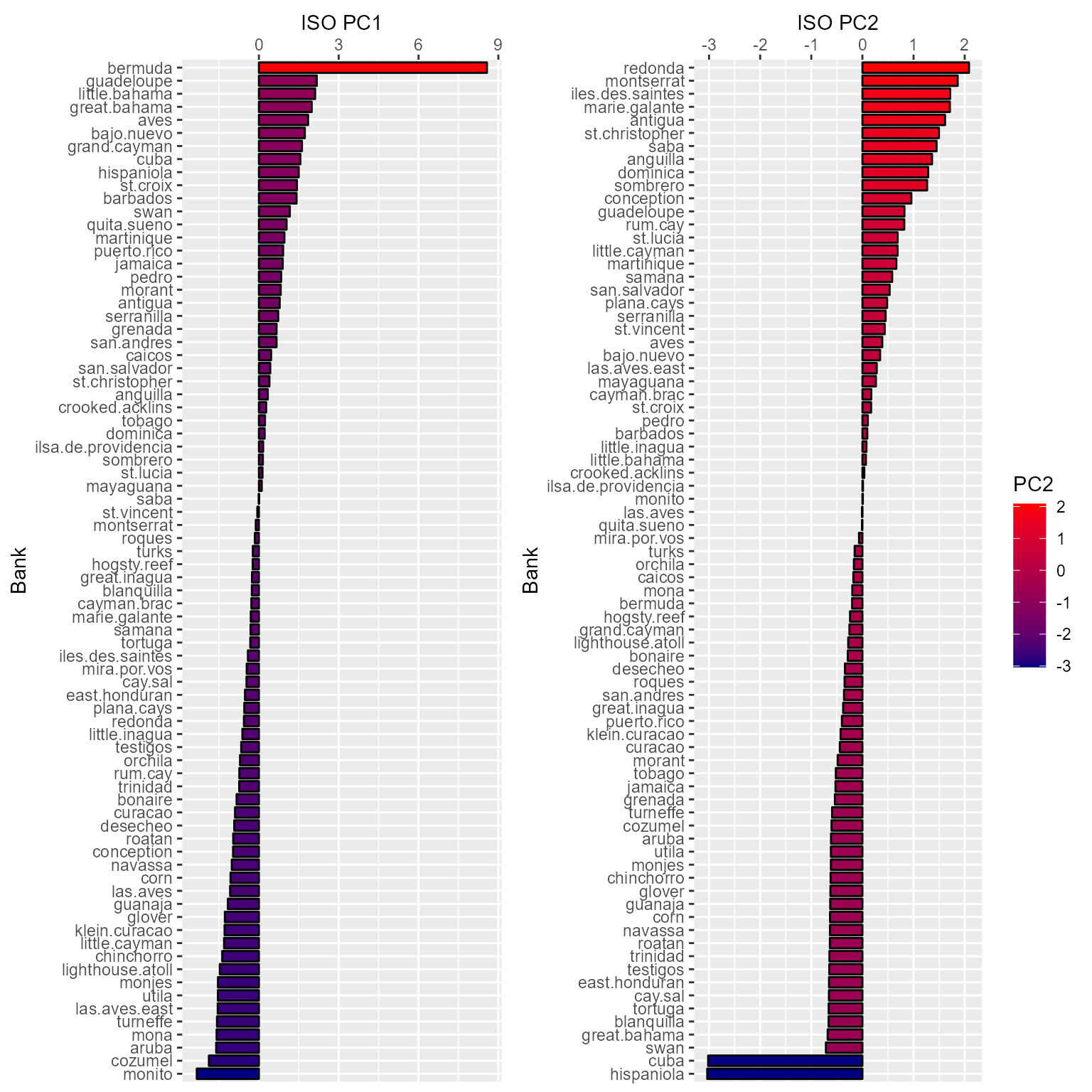
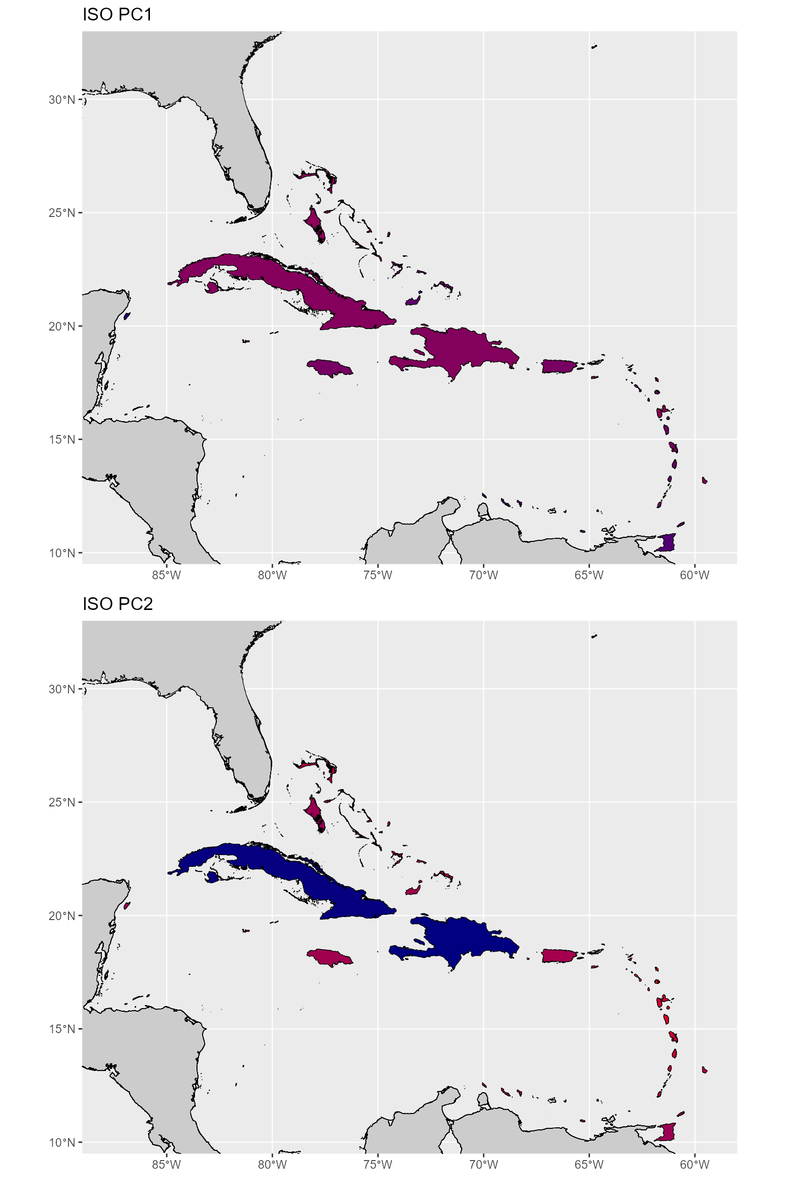
From these plots, the metrics do seem to make overall sense. However, there are clearly some outliers (Bermuda for PC1 and Cuba and Hispaniola for PC2). Additionally, Bermuda, which should be the most isolated for both PC1 and PC2, is considered less isolated from a source than most (if not all) the Lesser Antilles.
Therefore, it may make sense to just use the actual distances (square root transformed) as our metrics for isolation. This is especially true since we are only using three distances in the PCA anyway. First let’s see just how correlated all of the possible distances are so that we can see if we will have any collinearity issues in our analyses.
##           sum   min   main source larger
## sum     1.000 0.228 -0.554  0.022  0.087
## min     0.228 1.000  0.213  0.321  0.816
## main   -0.554 0.213  1.000  0.566  0.334
## source  0.022 0.321  0.566  1.000  0.383
## larger  0.087 0.816  0.334  0.383  1.000
The only distances that have a correlation over 0.6 is the distance to a larger bank and the distance to nearest bank. So we could use any of the others and either one of the ones that are highly correlated. Let’s select the distance to a source, nearest bank, and the mainland for right now and see how these values are distribute across the banks.
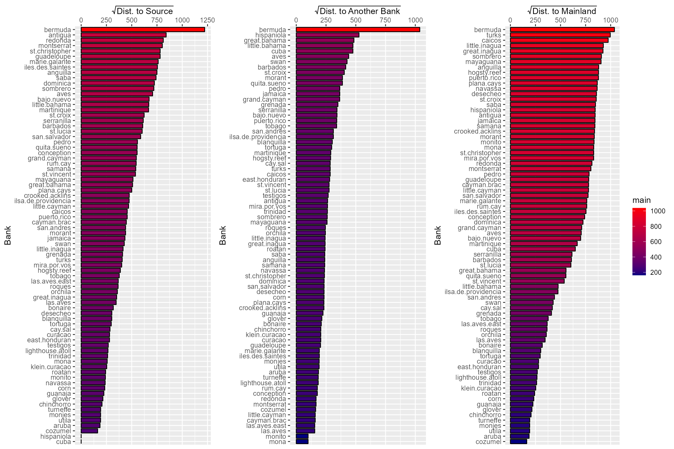
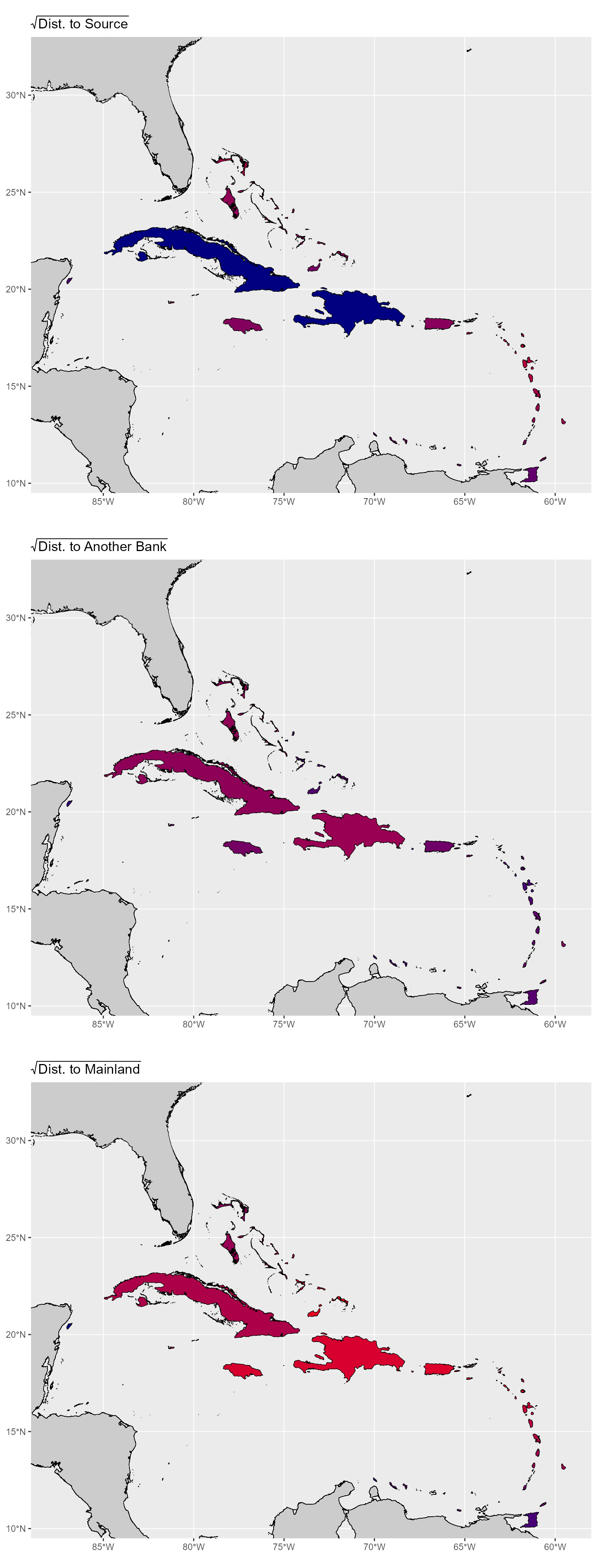
From these plots we can see that these distances tell us exactly what we want to show with our isolation metrics without any strange things happening for particular island banks. Additionally, we can see that the distance to nearest bank and distance to a source both approximately mirror PC1 (r = 0.91) and PC2 (r = 0.79), respectively. That means that if we run into issues where the slight correlation between our distances muddies any relationship we see, we can always use the PCs as isolation metrics.
Bank Economic Data
Now we will read in the banks’ economic data. These data are the number of shipment to and from various Caribbean banks as recorded by Lloyd’s of London for 4 separate years (1979, 1991, 2003, and 2015).
We will also be using population estimates for each bank from the Gridded Population of the World Version 4.11 (DOI: 10.7927/H4JW8BX5). The Gridded Population data set includes estimates of population counts for 30 arc-second pixels for the years 2000, 2005, 2010, 2015, and 2020. The estimates for the Caribbean banks were extracted using Google Earth Engine (JavaScript scripts can be found at the project GitHub page). We then will take the average of the five years of estimates and use that in our analyses.
For these data we will assume that any NA values
represent zeros. In the dataset, an NA means that there was
no recorded visits to that particular bank by a vessel tracked by
Lloyd’s. Therefore, assuming that NA values represent zeros
is valid when only considering vessels tracked by by Lloyd’s. The
acceptability for of this for bank population may not be as good given
that some of the banks may have land areas less than a 30 arc-second
pixel, and therefore, no data was extracted for that bank. However,
given the size of these banks, it is likely that the permanent
populations of the banks are very small if not zero.
To determine the maximum number of ships for each bank we will have
to use another function created for the ‘caribmacro’ package. This
function is row_max() and calculates the maximum value in
each row of a data frame.
bank_e <- read.csv(file.path(here(), 'data_raw', 'IBT_Lloyd_Bank_Degree_v0.csv'), header = TRUE)
bank_e <- bank_e[, c("bank", "to_1979", "to_1991", "to_2003", "to_2015", "to_total")]

for (i in 1:ncol(bank_e)) {
  bank_e[is.na(bank_e[, i]), i] <- 0
}

bank_e$ships_avg <- rowMeans(bank_e[, c("to_1979", "to_1991", "to_2003", "to_2015")], na.rm = TRUE)
bank_e$ships_max <- row_max(bank_e[, c("to_1979", "to_1991", "to_2003", "to_2015")], na.rm = TRUE)

names(bank_e)[which(names(bank_e) == 'to_total')] <- 'ships'
bank_e$bank <- as.factor(bank_e$bank)

pop <- read.csv(file.path(here(), 'data_raw', 'IBT_Bank_Population_v0.csv'), header = TRUE)

bank_e <- merge(bank_e, pop, by = 'bank', all = TRUE)

econ <- bank_e[, c('bank', 'ships', 'pop_avg')]## ships ships_avg ships_max
## ships 1.0000000 1.0000000 0.9771492
## ships_avg 1.0000000 1.0000000 0.9771492
## ships_max 0.9771492 0.9771492 1.0000000Since the maximum, average, and total number of ships that visited each bank during those four years are all correlated with each other we will just use the total number of ships since it is a better representation of the possibility of species introductions due to trade in recent history.
Let’s look at the distribution of some of these variables.
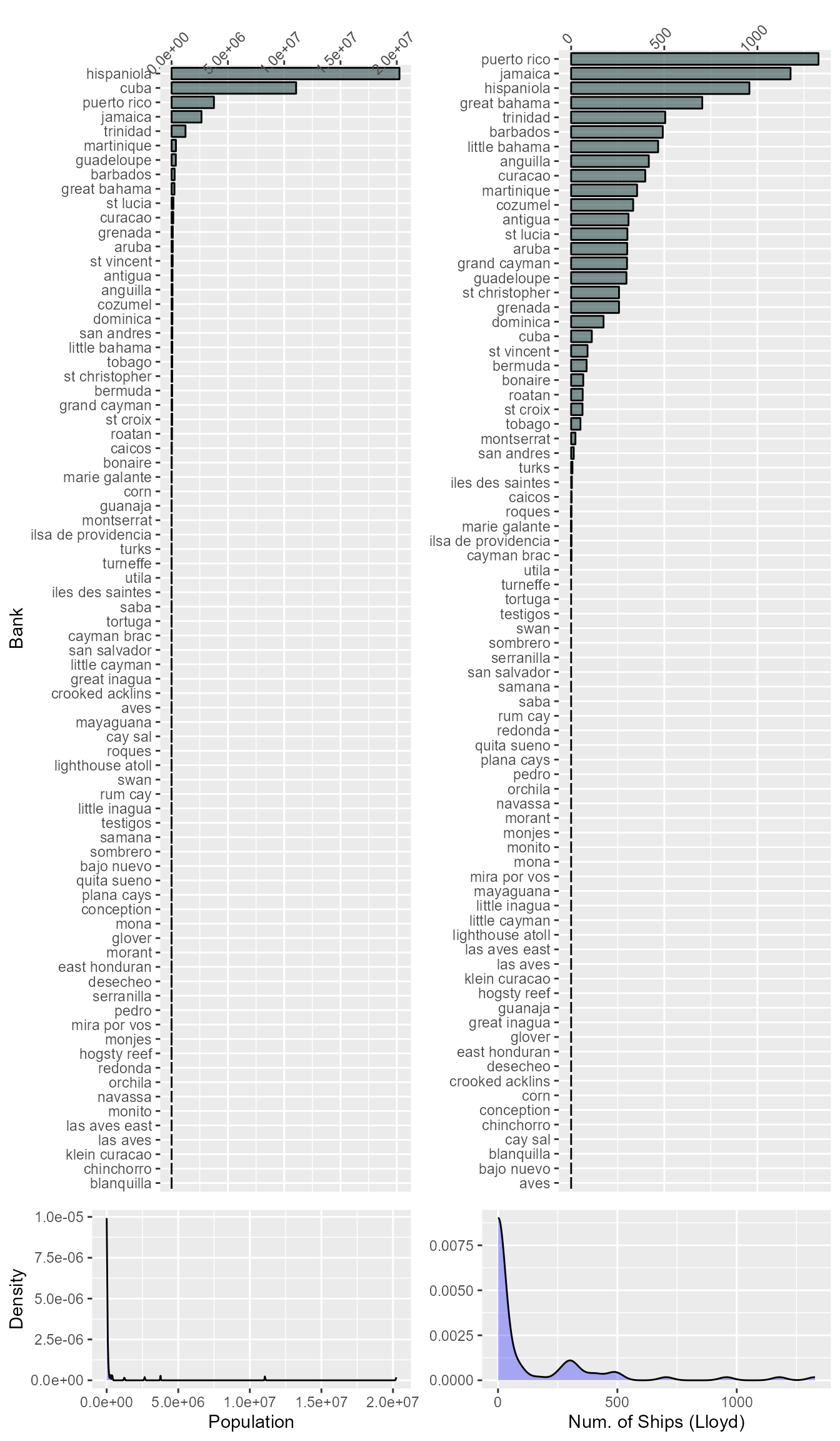
Bank Data
Now let’s combine all of the bank data into a single data frame.
X$bank <- gsub(' ', '.', X$bank)
bank_dat <- merge(X, iso[['Components']][, c('bank', 'PC1', 'PC2')], by = 'bank', all = TRUE)
names(bank_dat)[which(names(bank_dat) == 'PC1' | names(bank_dat) == 'PC2')] <- c('iso.PC1', 'iso.PC2')

bank_dat <- merge(bank_dat, iso[['Distances']][, c('bank', 'min', 'main', 'source')], by = 'bank', all = TRUE)

lndcvr$bank <- gsub(' ', '.', lndcvr$bank)
bank_dat <- merge(bank_dat, lndcvr, by = 'bank', all = TRUE)

econ$bank <- gsub(' ', '.', econ$bank)
bank_dat <- merge(bank_dat, econ, by = 'bank', all = TRUE)
The bank_dat data frame now holds all of the data we may
need for the island biogeographic analysis and needs to be exported to
the ‘data_out’ folder. Additionally, we should export the information of
the isolation PCAs to the ‘supp_info’ folder in the ‘data_out’ folder.
Once these data are exported, we can then remove the objects loaded into
R for the determination of the bank attributes.
write.csv(bank_dat, file.path(here(), 'data_out', 'IBT_Bank_Data.csv'), row.names = FALSE)

write.csv(iso[['Variance']], file.path(here(), 'data_out', 'supp_info', 'IBT_ISO_PCA_Var.csv'), row.names=FALSE)
write.csv(iso[['Loadings']], file.path(here(), 'data_out', 'supp_info', 'IBT_ISO_PCA_Load.csv'), row.names=FALSE)
Temple University, jmg5214@gmail.com↩︎