Get GBIF Records • slfrsk

Obtain Coordinate Data from GBIF for SLF and TOH

This vignette shows how we obtained the most recent version of data for SLF and TOH coordinates and then cleaned said data for use in SDMs.

Setup

We first loaded the full suite of required libraries. The most critical for this particular vignette is spocc, which is the package that allows us to query GBIF (Global Biodiversity Information Facility).

library(slfrsk) #this package, has extract_enm()
library(tidyverse)  #data manipulation
library(here) #making directory pathways easier on different instances
library(spocc) #query gbif and format as a dataframe
library(scrubr) #clean records for gbif data
library(humboldt) #rarefy points
library(tcltk) #humboldt progress bar
library(patchwork) #easy combined plots

Acquire and Clean Data

Acquire Data

We perform initial queries from GBIF for both SLF and TOH. We set the limit on records to be \(10^5\) to capture all TOH records (after an initial test query). Notably, we also limit records to those with coordinates, given our purpose for these data. Our queries use the accepted latin binomial nomenclature for both species.

It bears warning that the TOH query takes a considerable amount of time (\(>120s\)). We have it turned off by default (See below for more infomation).

if(FALSE){
  
#query for both species from gbif with limit of queries to 10^5
slf_gbif <- occ(query = 'Lycorma delicatula', from = 'gbif', limit = 1e5, has_coords = TRUE, throw_warnings = TRUE)
toh_gbif <- occ(query = 'Ailanthus altissima', from = 'gbif', limit = 1e5, has_coords = TRUE, throw_warnings = TRUE)

}

We then turn the raw output into dataframes via as_tibble(). Oddly, this function fails to strip list items from the TOH data, so we set that particular subset to NULL afterwards to fully flatten the TOH dataset. These results could then be saved for reference/reproducibility and are ultimately called by this vignette to save run time.

We end up also saving a copy of the coordinate results that have been transformed with spocc::occ2df() as well. The output of this function is a cleaner dataframe that we manipulate for the rest of the vignette.

if(FALSE){
  
#tibble the raw queries for saving
slf_gbif_final <- as_tibble(slf_gbif$gbif$data$Lycorma_delicatula)
toh_gbif_final <- as_tibble(toh_gbif$gbif$data$Ailanthus_altissima)

#de-listify TOH
toh_gbif_final$networkKeys <- NULL

#save the raw queries with the date stamp for current date
write_csv(x = slf_gbif_final, file = file.path(here(), "data-raw", paste0( "slf_gbif_", format(Sys.Date(), "%Y-%d-%m"), ".csv")))
write_csv(x = toh_gbif_final, file = file.path(here(), "data-raw", paste0( "toh_gbif_", format(Sys.Date(), "%Y-%d-%m"), ".csv")))

#turn occ data into df
slf_coords1 <- occ2df(slf_gbif)
toh_coords1 <- occ2df(toh_gbif)

#save the coords as they are
write_csv(x = slf_coords1, file = file.path(here(), "data-raw", paste0( "slf_gbif_raw_coords_", format(Sys.Date(), "%Y-%d-%m"), ".csv")))
write_csv(x = toh_coords1, file = file.path(here(), "data-raw", paste0( "toh_gbif_raw_coords_", format(Sys.Date(), "%Y-%d-%m"), ".csv")))

}

Here is where we read in the raw data queried for this study:

#read in raw data
slf_coords1 <- read_csv(file = file.path(here(), "data-raw", "slf_gbif_raw_coords_2020-20-10.csv"))
toh_coords1 <- read_csv(file = file.path(here(), "data-raw", "toh_gbif_raw_coords_2020-20-10.csv"))

Clean Data

Now we can proceed to clean the data for use. We clean the data in three regards:

consistent taxonomic labels
coordinate veracity
coordinate rarefication

Consistent Taxonomy

Firstly, we check for taxonomic consistency in each dataset. Spoiler: SLF is fine and TOH needs to be homogenized. Thankfully, a check of the GBIF page for TOH (https://www.gbif.org/species/3190653) shows that all of the other names are just junior synonyms. Therefore, we change all of them to the same taxonomy.

#check the taxonomy for only correct queries
unique(slf_coords1$name) #all the same
#> [1] "Lycorma delicatula (White, 1845)"
unique(toh_coords1$name)
#> [1] "Ailanthus altissima (Mill.) Swingle"                              
#> [2] "Ailanthus altissima var. altissima"                               
#> [3] "Ailanthus altissima var. tanakai (Hayata) Kanehira & Sasaki"      
#> [4] "Ailanthus glandulosa Desf."                                       
#> [5] "Ailanthus giraldii Dode"                                          
#> [6] "Ailanthus vilmoriniana Dode"                                      
#> [7] "Ailanthus altissima subsp. tanakai (Miller) Swingle"              
#> [8] "Ailanthus altissima subsp. altissima"                             
#> [9] "Ailanthus altissima var. sutchuenensis (Dode) Rehder & E.H.Wilson"

#toh data contains a bunch of synonyms according to GBIF (https://www.gbif.org/species/3190653)
#therefore, we are going to make them all the same, the top species designation
toh_coords1$name <- "Ailanthus altissima (Mill.) Swingle"

Coordinate Veracity

Coordinate veracity has several components that amount to removing coordinates that do not make sense. Given the difference in raw records for both species, SLF is easily cleaned of dubious records while TOH has too many records and breaks at least one function (scrubr::dedup()) if run through the cleaning steps with removal of duplicates before rarefication. To account for this, both datasets run scrubr::dedup() after rarefication.

We make good use of the scrubr package functions to clean coordinates.

slf_coords1 <- slf_coords1 %>%
  coord_incomplete() %>%  #rm incomplete coords, those that lack valid lat and long
  coord_impossible() %>% #rm impossible coords, those that are not possible (e.g., lat > 90)
  coord_unlikely()  #rm unlikely coords, such as those at 0,0
#> Assuming 'latitude' is latitude
#> Assuming 'longitude' is longitude

#toh
toh_coords1 <- toh_coords1 %>%
  coord_incomplete() %>%  #rm incomplete coords, those that lack valid lat and long
  coord_impossible() %>% #rm impossible coords, those that are not possible (e.g., lat > 90)
  coord_unlikely()      #rm unlikely coords, such as those at 0,0
#> Assuming 'latitude' is latitude
#> Assuming 'longitude' is longitude

Coordinate Rarefication

We now use the humboldt package rarefaction function humboldt::humboldt.occ.rarefy() to trime points that are \(<10 km\) from each other. This cleaning step reduces spatial autocorrelation in our data, which is a good thing! After this, we run the data through scrubr::dedup.

Note that the rarefaction takes a while for TOH especially (it is cleaning 67000+ records after all). We also manually remove some points from SLF that are clearly incorrect as of Fall 2020 (after consulting colleagues).

if(FALSE){
  
#rarefy points
slf_coords2 <- humboldt.occ.rarefy(in.pts = slf_coords1, colxy = 2:3, rarefy.dist = 10, rarefy.units = "km", run.silent.rar = F)
toh_coords2 <- humboldt.occ.rarefy(in.pts = toh_coords1, colxy = 2:3, rarefy.dist = 10, rarefy.units = "km", run.silent.rar = F)

#dedup now
slf_coords3 <- slf_coords2 %>%
  dedup(how = "one", tolerance = 0.99)
toh_coords3 <- toh_coords2 %>%
  dedup(how = "one", tolerance = 0.99)

#rm manually incorrect SLF points
#we have points in: MA, NE, OR, DE coast for SLF that need to be removed
#key should work to get rid of identified points
slf_coords3 <- slf_coords2 %>%
  filter(key != "2860187641") %>% #rm OR---lat, lon:(43.63691, -121.85569)
  filter(key != "2862292948") %>% #rm NE---lat, lon:(42.50641,-101.01562)
  filter(key != "2864687343") %>% #rm DE---lat, lon:(37.91855, -75.14999)
  filter(!key %in% c("2856537682", "2851117559")) #rm MA---lat, lon: (42.20994, -71.18331)

#change order of final coords to be lat, lon
slf_coords3 <- slf_coords3 %>%
  dplyr::select(name, latitude, longitude, prov, date, key)
toh_coords3 <- toh_coords3 %>%
  dplyr::select(name, latitude, longitude, prov, date, key)

#write the saved final data
write_csv(slf_coords3, file = file.path(here(), "data-raw", "slf_gbif_cleaned_coords_2020.csv"))
write_csv(toh_coords3, file = file.path(here(), "data-raw", "toh_gbif_cleaned_coords_2020.csv"))

}

Visualize Data

We can read in the final data for looking at the spatial coverage despite the thinning.

#read in data for viewing differences
#slf_coords3 <- read_csv(file = file.path(here(), "data-raw", "slf_gbif_cleaned_coords_2020.csv"))
#toh_coords3 <- read_csv(file = file.path(here(), "data-raw", "toh_gbif_cleaned_coords_2020.csv"))

#note: we read in slightly modified versions of the same coords. lat/lon were changed to y/x respectively and the species names were cleaned up. see corresponding section in data-raw/convert_data_rda.R for details
data("slf_points", package = "slfrsk")
data("toh_points", package = "slfrsk")

#plot the difference
#TOH
map_toh <- ggplot() +
  geom_polygon(data = map_data('world'), aes(x = long, y = lat, group = group), fill = NA, color = "black", lwd = 0.15) +
  geom_point(data = toh_coords1, aes(x = longitude, y = latitude), color = "red", size = 2) +
  geom_point(data = toh_points, aes(x = x, y = y), color = "blue", shape = 2) +
  coord_quickmap(xlim = c(-164.5, 163.5), ylim = c(-55,85)) +
  ggtitle("TOH") +
  theme(panel.grid.major = element_blank(),
        panel.grid.minor = element_blank(),
        panel.background = element_blank()) +
  theme_bw()
#SLF
map_slf <- ggplot() +
  geom_polygon(data = map_data('world'), aes(x = long, y = lat, group = group), fill = NA, color = "black", lwd = 0.15) +
  geom_point(data = slf_coords1, aes(x = longitude, y = latitude), color = "red", size = 2) +
  geom_point(data = slf_points, aes(x = x, y = y), color = "blue", shape = 2) +
  coord_quickmap(xlim = c(-164.5, 163.5), ylim = c(-55,85)) +
  ggtitle("SLF") +
  theme(panel.grid.major = element_blank(),
        panel.grid.minor = element_blank(),
        panel.background = element_blank()) +
  theme_bw()

#patchwork output of both maps
map_toh / map_slf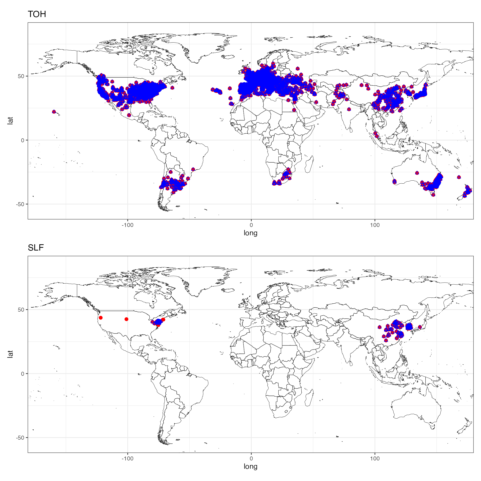

We have practically the same coverage with less autocorrelation (note the dropped false records for SLF)! Now we can use these data for SDMs!