Paninvasion Risk
vignette-041-market-plot.RmdQuantify Paninvasion Risk to Shock Wine Market
This vignette aims to reproduce the published figure(s) of the relationship between the predicted production of grapes from a severity model built from the alignment of the three invasion potentials (impact potential regressed on transport and establishment) to the wine market share by country.
Load and summarize data
Market size data
Next, we read in the countries_market dataset, which
contains exports of wine by country. The data are in
thousands of USD (1000’s USD), and so we will need to convert to USD as
we summarize the data. We summarize the market data by
obtaining the mean of \(log_{10}(value+1)\) transformed export
values from 2012–2017.
We quickly visualize the distribution of these summarized
market_size data via a histogram:
data("countries_market")
#dim(countries_market)

# http://www.fao.org/faostat/en/#data/TM
countries_wine_market <- countries_market %>%
  filter(Year %in% (2012:2017)) %>%
  filter(Element == "Export Value") %>%
  group_by(`Area Code`, Area, Year) %>%
  dplyr::select(`Area Code`,    Area, Year, Value) %>%
  summarise(market_size = sum(Value)) %>%
  ungroup(Year) %>%

  mutate(market_size = log10((market_size*1000)+1)) %>% # units are in 1000s of USD
  #mutate(market_size = (market_size*1000)) %>%
  summarise(market_size = mean(market_size))  %>%
  ungroup()

# remove all that are zero

countries_wine_market$market_size[countries_wine_market$market_size==0] <- NA
#countries_wine_market$market_size <- round(countries_wine_market$market_size)

#dim(countries_wine_market)
#countries_wine_market

qplot((countries_wine_market$market_size))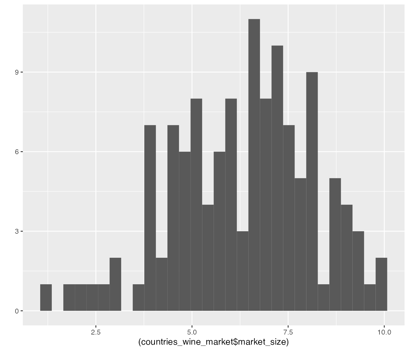
From here, we add an ID column that matches the other
use of this label in the other package vignettes. Then, we isolate
ID and market_size for risk analyses.
Market summary data
To merge the new market_size dat with our existing
countries data, we use left_join() to merge
the market and summary data by
ID. We then remove the countries from the dataset that
already have SLF. Note: we use a modified version of
%in% and Negate() to create
%notin% for removing countries.
#data("countries_summary_present")
data("countries_summary_present_ensemble")
countries_summary_present_ensemble <- countries_summary_present_ensemble %>%
    filter(!ID %in% c("Antarctica", "Monaco", "Norfolk Island", "Spratly Islands"))

#remove non-focal countries
rems <- c("Akrotiri and Dhekelia"
            ,"?land"
            ,"American Samoa"
            ,"Bouvet Island"
            ,"British Indian Ocean Territory"
            ,"Caspian Sea"
            ,"Christmas Island"
            ,"Clipperton Island"
            ,"Cocos Islands"
            ,"Falkland Islands"
            ,"Faroe Islands"
            ,"French Southern Territories"
            ,"Heard Island and McDonald Islands"
            ,"Mayotte"
            ,"Northern Mariana Islands"
            ,"Paracel Islands"
            ,"Pitcairn Islands"
            ,"Saint Pierre and Miquelon"
            ,"Tokelau"
            ,"United States Minor Outlying Islands"
            ,"Wallis and Futuna"
            ,"United States"
            ,"Philippines")

countries_summary_present_ensemble <- countries_summary_present_ensemble %>% filter(!ID %in% rems)


#dim(countries_summary_future)
`%notin%` <- Negate(`%in%`)

# filter(countries_summary_future, status == "native")

countries_sev_market <- countries_summary_present_ensemble %>%
  left_join(countries_wine_market, by = "ID") %>%
  filter(ID %notin% c("United States",
                      "China",
                      "India",
                      "Taiwan",
                      "Japan",
                      "South Korea",
                      "Vietnam"))#%>%

#########
# - Use this code to check to make sure that each country only has one row
# dim(countries_sev_market)
# setdiff(countries_sev_market$ID,countries_summary_future$ID)
# setdiff(countries_summary_future$ID,countries_sev_market$ID)
# table(countries_sev_market$ID)[table(countries_sev_market$ID)>1]
# table(countries_summary_future$ID)[table(countries_summary_future$ID)>1]
Build and check model
From here, we now can build (or rebuild, technically,
vignette-021-quadrant-plots does this first part as well)
the severity model (sev_mod). This model is a linear
regression model of log-transformed impact potential on
the log-transformed transport and normal
establishment potentials. We then evaluated the
strength of the correlation between the empirical and predicted
impact potential before conducting some
diagnostics.
We then rescaled the predicted impact values to be
bounded \([1,10]\) to produce initial
sev values.
To create the initial shock model (shock_mod)
and ultimately obtain a scaled measure of risk of SLF
to shock the global wine market, we performed linear regression of the
market_size data on sev for countries and
conducted diagnostics as for sev_mod. We then evaluated the
unscaled and scaled correlations between market_size and
sev for countries, resulting in a risk of \(8\) based on a scale of \([1,10]\).
sev_mod <- lm(log10_avg_prod ~ log10_avg_infected_mass + grand_mean_max,
               data = countries_sev_market)
cor.test(countries_sev_market$log10_avg_prod, predict(sev_mod), method = "spearman")
#> Warning in cor.test.default(countries_sev_market$log10_avg_prod,
#> predict(sev_mod), : Cannot compute exact p-value with ties
#>
#>  Spearman's rank correlation rho
#>
#> data:  countries_sev_market$log10_avg_prod and predict(sev_mod)
#> S = 605845, p-value < 2.2e-16
#> alternative hypothesis: true rho is not equal to 0
#> sample estimates:
#>       rho
#> 0.6722015

## diagnostics
# fit is good for the multivariate correlation because there is no dispersion, but do not use this model for prediction (which I do not know why you would)
simulationOutput_r <- simulateResiduals(fittedModel = sev_mod, plot = T) 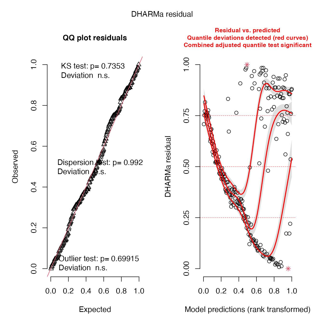
testDispersion(simulationOutput_r) 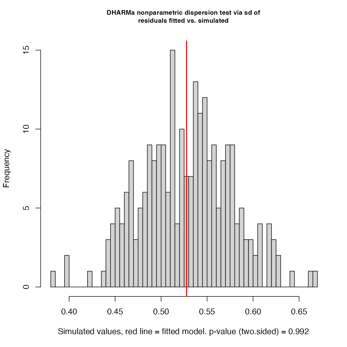
#>
#>  DHARMa nonparametric dispersion test via sd of residuals fitted vs.
#>  simulated
#>
#> data:  simulationOutput
#> dispersion = 0.99972, p-value = 0.992
#> alternative hypothesis: two.sided
summary(sev_mod)
#>
#> Call:
#> lm(formula = log10_avg_prod ~ log10_avg_infected_mass + grand_mean_max,
#>     data = countries_sev_market)
#>
#> Residuals:
#>     Min      1Q  Median      3Q     Max
#> -4.4760 -1.0949 -0.0788  1.1946  4.8336
#>
#> Coefficients:
#>                         Estimate Std. Error t value Pr(>|t|)
#> (Intercept)             -1.20443    0.26085  -4.617 6.61e-06 ***
#> log10_avg_infected_mass  0.36455    0.06576   5.544 8.44e-08 ***
#> grand_mean_max           4.44430    0.44357  10.019  < 2e-16 ***
#> ---
#> Signif. codes:  0 '***' 0.001 '**' 0.01 '*' 0.05 '.' 0.1 ' ' 1
#>
#> Residual standard error: 1.732 on 220 degrees of freedom
#> Multiple R-squared:  0.4788, Adjusted R-squared:  0.4741
#> F-statistic: 101.1 on 2 and 220 DF,  p-value: < 2.2e-16

countries_sev_market <- countries_sev_market %>%
  mutate(sev = scales::rescale(predict(sev_mod), to = c(1,10)))

shock_mod <- lm(market_size ~ sev, data = countries_sev_market)
summary(shock_mod)
#>
#> Call:
#> lm(formula = market_size ~ sev, data = countries_sev_market)
#>
#> Residuals:
#>     Min      1Q  Median      3Q     Max
#> -3.9202 -0.7753  0.0795  0.8965  3.6390
#>
#> Coefficients:
#>             Estimate Std. Error t value Pr(>|t|)
#> (Intercept)  2.46385    0.36445    6.76 8.75e-10 ***
#> sev          0.61487    0.05503   11.17  < 2e-16 ***
#> ---
#> Signif. codes:  0 '***' 0.001 '**' 0.01 '*' 0.05 '.' 0.1 ' ' 1
#>
#> Residual standard error: 1.249 on 102 degrees of freedom
#>   (119 observations deleted due to missingness)
#> Multiple R-squared:  0.5503, Adjusted R-squared:  0.5459
#> F-statistic: 124.8 on 1 and 102 DF,  p-value: < 2.2e-16

## diagnostics
# severity estimate model fit is good and no major issues in heteroskedasticity. But I am not certain why you want this model anyways, a correlation is better because it is easily scaled between 1-10
simulationOutput <- simulateResiduals(fittedModel = shock_mod, plot = T) 
testDispersion(simulationOutput)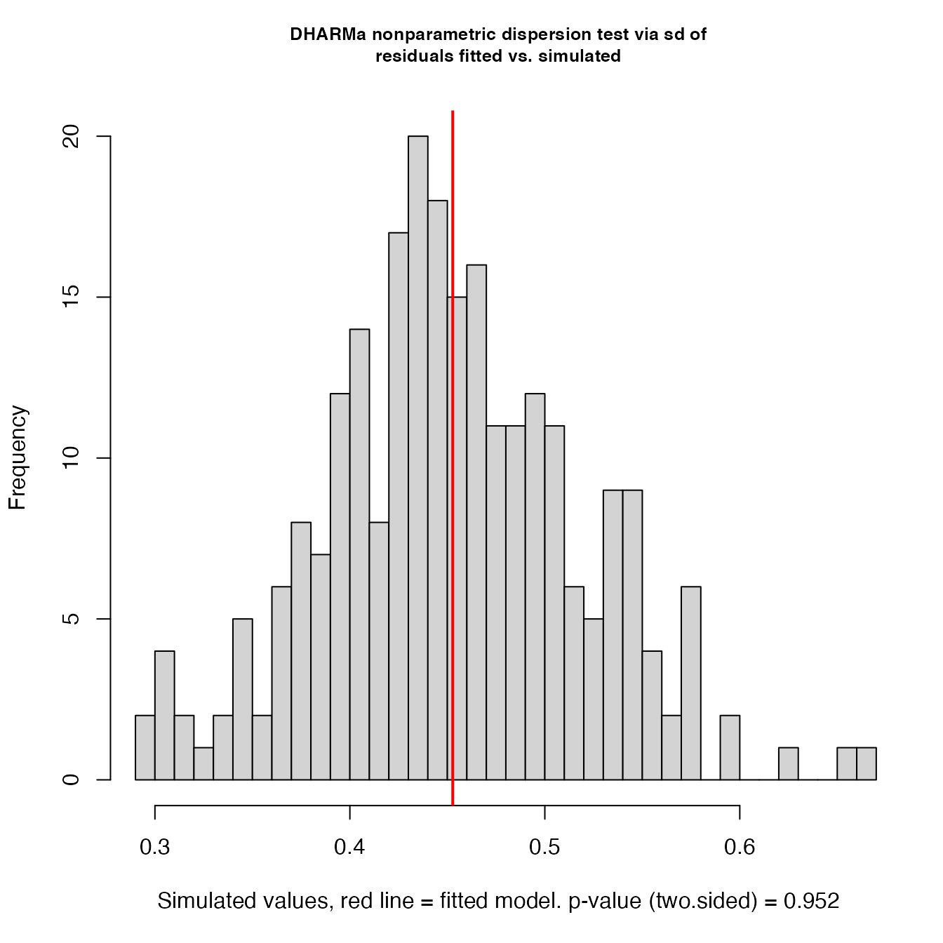
#>
#>  DHARMa nonparametric dispersion test via sd of residuals fitted vs.
#>  simulated
#>
#> data:  simulationOutput
#> dispersion = 1.0013, p-value = 0.952
#> alternative hypothesis: two.sided

cor.test(countries_sev_market$market_size, countries_sev_market$sev)
#>
#>  Pearson's product-moment correlation
#>
#> data:  countries_sev_market$market_size and countries_sev_market$sev
#> t = 11.173, df = 102, p-value < 2.2e-16
#> alternative hypothesis: true correlation is not equal to 0
#> 95 percent confidence interval:
#>  0.640816 0.817623
#> sample estimates:
#>       cor
#> 0.7418499
(shock_cor <- cor(countries_sev_market$market_size,
                 countries_sev_market$sev,
                 use = "complete.obs") %>%
  scales::rescale(to = c(1,10), from = c(-1,1)) %>%
  round())
#> [1] 9
Plotting risk vs market scatter
With the predicted risk, we were able plot the
scaled sev and market_size, resulting in the
published risk of SLF to shock the global wine market
plot.
Static plot
market_scatter <- countries_sev_market %>%

  ggplot(mapping = aes(x = (sev),
                       y = (market_size),
                       size = avg_wine,
                       fill = wine)
         ) +
  geom_abline(slope = 1, intercept = 0, lty = 2) +
  geom_abline(slope = 1, intercept = 5, lty = 2) +
  geom_abline(slope = 1, intercept = -5, lty = 2) +

  ggtitle(label = paste('Spotted Lanternfly Paninvasion Risk =',
                        shock_cor,'of 10 (P<0.001)')) +
  geom_point(pch = 21) +
     scale_x_continuous(
    name =  substitute(expr = paste('Spotted Lanternfly (',italic("Lycorma delicatula"),') Invasion Risk')),
    breaks = 1:10,
    limits = c(1,10)
    ) +
  scale_y_continuous("Wine Export Market Size, log10 USD",
                     breaks = seq(1,10,1),
                     limits = c(1,10)
                     ) +
  scale_size_continuous(
        #values = c(0,),
       name = "Wine Production",# "Wine Impact Potential",
       # labels = c("0 t", "1.0M t", "2.0M t", "3.0M t", "4.0M t")
        labels = c("0 t", "1E6 t", "2E6 t", "3E6 t", "4E6 t")

      ) +
 # scale_fill_discrete(guide = FALSE) +
   scale_fill_manual(
         values = c("no" = "#ffffff", "yes" = "#C77CFF"),
         name = "",# "Wine Impact Potential",
         labels = c("wine producer", "")
       ) +
      theme(
        panel.grid.major = element_line(colour = "#f0f0f0"),
        panel.grid.minor = element_blank(),
        #panel.grid.major = element_blank(),
        #panel.border = element_rect(colour = "black", fill=NA, size=1),
        axis.line = element_line(colour = "black"),
        #legend.position = c(0.7, 0.25),
        #legend.position = "bottom",
        panel.background = element_blank(),
        plot.background = element_blank(),
        #legend.background = element_rect(colour = 'black',
        #                                 fill = 'white',
        #                                 linetype='solid'),
        axis.text = element_text(size = rel(1)),
        axis.title.x = element_text(hjust = .4),
        axis.title.y = element_text(hjust = .35),
        legend.title = element_text(face = "plain"),
        legend.key.size = unit(0.2, "cm"),
        legend.key = element_blank(),
        #plot.margin = unit(c(hh, -5, hh, hh), units = "line"),
        #axis.title = element_text(size = rel(1.3))
      ) +
  geom_text_repel(#data = select(countries_sev_market,
                      aes(#x = x_to_plot,
                          #y = y_to_plot,
                          label = ID),
                      #label = countries_sev_market$ID,
                      min.segment.length = 0,
                      #direction = "x",
                      #nudge_y = nudge.y,
                      #nudge_x = nudge.x
      show.legend = FALSE) #+
  #guides(
  #      fill = TRUE
  #      ) #,
      #   color = guide_legend(
      #     order = 3,
      #     override.aes = list(alpha = 1)
      #   ),
      #   size = guide_legend(    # Adjust size to edit legend grape production
      #     order = 2,            # circles.
      #     override.aes = list(size = c(1,3,6), alpha = 1)
      #   )
      # )

market_scatter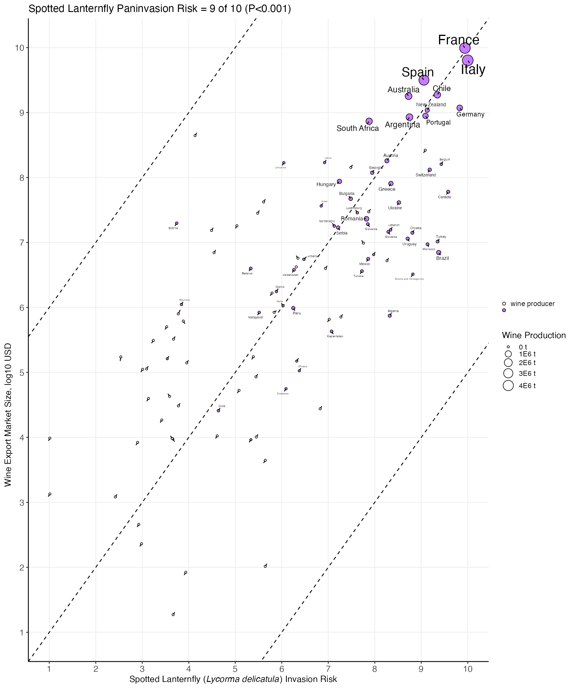
Interactive plot
We also provide an interactive version of the risk plot with
plotly.
#build ggplot
p1 <- countries_sev_market %>%
  mutate_if(.predicate = is.numeric, .funs = ~round(x = ., digits = 2)) %>%
    ggplot(mapping = aes(x = sev,
                       y = market_size,
                       size = avg_wine,
                       fill = wine
                       )
         ) +
  geom_abline(slope = 1, intercept = 0, lty = 2) +
  geom_abline(slope = 1, intercept = 5, lty = 2) +
  geom_abline(slope = 1, intercept = -5, lty = 2) +
  geom_point(pch = 21, aes(text = ID)) +
  scale_fill_manual(
         values = c("no" = "#ffffff", "yes" = "#C77CFF"),
         name = "",
         labels = c("wine producer", "")
       ) +
  lims(x = c(1, 10), y = c(1, 10)) +
  theme(
        panel.grid.major = element_line(colour = "#f0f0f0"),
        panel.grid.minor = element_blank(),
        axis.line = element_line(colour = "black"),
        panel.background = element_blank(),
        plot.background = element_blank(),
        axis.text = element_text(size = rel(1)),
        axis.title.x = element_text(hjust = .4),
        axis.title.y = element_text(hjust = .35),
        legend.title = element_text(face = "plain"),
        legend.key.size = unit(0.2, "cm"),
        legend.key = element_blank(),
      )

#execute plotly
ggplotly(p = p1, tooltip = c("ID", "sev", "market_size", "wine"), dynamicTicks = T) %>%
layout(xaxis =
           list(title = list(text = paste('Spotted Lanternfly',sprintf("(<i>Lycorma delicatula</i>)"),'Invasion Risk'), font = list(size = 11)), showspikes = T),
         yaxis =
           list(title = list(text = "Wine Export Market Size, log10 USD", font = list(size = 11)), showspikes = T),
         title =
           list(text = paste('Spotted Lanternfly Paninvasion Risk =', shock_cor,'of 10 (P<0.001)'),
                font = list(size = 12),
                x = 0.1,
                y = 0.99),
         showlegend = F
         )
Save plot output
Here, you can set to save the scatter plot to /vignettes
as a .pdf file by setting the if from
FALSE to TRUE, as in the other vignettes. We
also have a version of the data saved for the Google Earth Engine App
data cleaning vignette.
if(FALSE){
  pdf(file.path(here::here(),
              "vignettes",
              paste0("market_scatter_v4_1.pdf")),
    width = 8.5*.95, height = 11*.95)

market_scatter
invisible(dev.off())

countries_sev <- countries_sev_market %>%
  dplyr::select(ID, market_size, sev)

save(countries_sev, file = file.path(here::here(), "data", "countries_sev.rda"))
}