Paninvasion Severity App
vignette-040-ee-data.RmdGoogle Earth Engine Paninvasion Severity App Companion: https://ieco.users.earthengine.app/view/ieco-slf-riskmap
Huron, N. A., Behm, J. E. & Helmus, M. R. 2022. Paninvasion severity assessment of a U.S. grape pest to disrupt the global wine market. Communications Biology, 5:1–11. https://doi.org/10.1038/s42003-022-03580-w.
Map Legend
The slrsk Paninvasion Severity App is an interactive map
that allows for highly customizable visualization. When loaded, it will
display a map of the earth with several different data layers already
enabled (see image below for example).

Landing page and labeled visualization tools for
slfrsk Paninvasion Severity App.
Map Widgets
The image shows several key tools that allow for interactive visualization. They are as follows:
- Zoom tool: can be used to zoom in (+) and zoom out (-)
- Annotation tools: allows for geographic annotation of points, lines, and polygons by the user. The hand icon returns to normal navigation.
- Location search bar: allows for navigating to a particular geographic region and functions similarly to searching on any GPS/navigation system.
- Layers panel: allows for toggling visibility on/off via check boxes
or changing opacity (alpha) of
slfrsklayers. See layers legend section below for further details on individual layers. - Explore Geographic Focus: dropdown menu that allows for exploring key geographic regions
- WRD: whole world view
- PHL: Philadelphia metro regional view
- ITA: northern Italy grape-growing view
- FRA: southern France grape-growing view
- ESP: northern Spain grape-growing view
- CAL: norhtern California grape-growing view
- ERA: Eurasian grape-growing view
- Establishment Potential Threshold: manually change the threshold of SLF establishment suitability (scaled [0,1]) such that values closer to 1 plot only the most suitable areas and values close to 0 plot closer to the full range of suitability.
- Legend Help link: clicking this link will direct back to this article (https://ieco-lab.github.io/slfrsk/articles/vignette-040-ee-data.html)
Layers Panel
The layers panel contains several key measures of SLF invasion potential. Each layer can be turned on or off via the checkbox to the left of its name. Additionally, the opacity of each layer can be changed via the slider bar to the right of its name. Below, we present a detailed account of each layer and its source data, as well as its color scale and geometry.

Default view of Layers Panel for slfrsk
Paninvasion Severity App.
- wine regions: important viticultural regions aggregated from the Tobacco Tax and Trade Bureau (TTB, Bureau (2019)) and Wikipedia (2020) are depicted by purple points
- vineyards EU: areas reported to be cultivated as vineyards in Europe according to Agency (2018) are depicted by purple pixels
- vineyards U.S: areas reported to be cultivated as vineyards in the U.S according to USDA National Agricultural Statistics Service (2019) are depicted by purple pixels
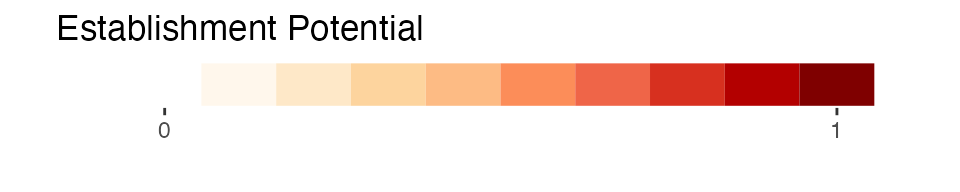
- establishment potential: the potential for establishment of SLF as determined from the suitability in the ensemble species distribution model (scaled \([0,1]\)). This layer is a shaded fill that goes with the Establishment Potential Threshold box discussed in the prior section.
- transport potential: the potential for transport of SLF as determined by the metric tonnage of trade with U.S states that are considered to have established SLF populations (scaled \([0,10]\)). This layer is a border outline for countries and U.S states.
![]()
-
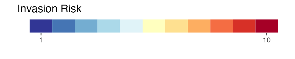
invasion risk: the severity of shock to the wine
market as determined by the relationship between predicted values of
average annual grape production based on SLF transport and establishment
potential and average annual wine market size (scaled \([1,10]\)). This scaling ranges from a
completely negative relationship at 1 to a completely positive
relationship at 10 (thus explaining the change from the \([0,10]\) scale seen for other layers) This
layer is a shaded fill for only
countriesthat do not already have established SLF populations.
Data preparation
This vignette is a companion to the interactive slfrsk
Google Earth Engine (EE) Paninvasion Severity App https://ieco.users.earthengine.app/view/ieco-slf-riskmap.
It provides a brief demonstration of how the data were treated prior to
inclusion in the app. Output data from this vignette are saved in the
shared GoogleDrive ./slfRiskMapping/data/slfrsk/
directory.
Setup
Here we load the packages that allow us to visualize color palettes
and reformat shapefile data and merge with the summarized potentials
data visualized in vignette-021-quadrant-plots.
Summary data
We then read in the summary data for both states and
countries from vignette-010-tidy-data to
eventually merge with shapfiles. We also remove any
countries with establishment potential that
are -Inf values.
#data("states_summary_future_ensemble")
#data("countries_summary_future_ensemble")
data("states_summary_present_ensemble")
data("countries_summary_present_ensemble")


#rm the -Inf countries
#countries_summary_future_ensemble <- countries_summary_future_ensemble %>%
#      filter(!ID %in% c("Antarctica", "Monaco", "Norfolk Island", "Spratly Islands"))
countries_summary_present_ensemble <- countries_summary_present_ensemble %>%
      filter(!ID %in% c("Antarctica", "Monaco", "Norfolk Island", "Spratly Islands"))
We now transform the summary data to represent scaled
versions of the three potentials (transport,
establishment, and impact). Each of
these potentials are saved in new columns: transport,
establishment, and two for impact
(impact_wine and impact_grape), which include
values for the corresponding potential that are \(\log_{10}(value+1)\) transformed and then
bounded \([0,10]\).
To bound these values, each \(\log\)-transformed value undergoes the following, based on the existing input data and round to a single digit for visualization:
- \(transport_{[0,10]} = \frac{transport - \min(transport)}{\max(transport)}*10\)
- \(establishment_{[0,10]} = establishment*10\)
- \(impact_{[0,10]} = \frac{impact}{\max(impact)}*10\)
After these transformations, we go ahead and round the raw data for reducing file size to 5 significant digits.
#states
states_summary_present_ensemble <- states_summary_present_ensemble %>%
  #transport in 2 mutate steps
  mutate(transport = log10_avg_infected_mass - min(log10_avg_infected_mass)) %>%
  mutate(transport = round(x = transport / max(transport), digits = 1)*10) %>%
  #establishment
  mutate(establishment = round(x = grand_mean_max, digits = 1)*10) %>%
  #impact_wine
  mutate(impact_wine = round(x = log10_avg_wine / max(log10_avg_wine), digits = 1)*10) %>%
  #impact_grape
  mutate(impact_grape = round(x = log10_avg_prod / max(log10_avg_prod), digits = 1)*10)

#rounding
states_summary_present_ensemble <- states_summary_present_ensemble %>%
  mutate(grand_mean_max = signif(grand_mean_max, digits = 5),
         #grand_se_max = signif(grand_se_max, digits = 5),
         avg_wine = signif(avg_wine, digits = 5),
         se_wine = signif(se_wine, digits = 5),
         log10_avg_wine = signif(log10_avg_wine, digits = 5),
         avg_yield = signif(avg_yield, digits = 5),
         se_yield = signif(se_yield, digits = 5),
         avg_prod = signif(avg_prod, digits = 5),
         se_prod = signif(se_prod, digits = 5),
         log10_avg_yield = signif(log10_avg_yield, digits = 5),
         log10_avg_prod = signif(log10_avg_prod, digits = 5),
         avg_infected_trade = formatC(signif(avg_infected_trade, digits = 5), format = "e"),
         se_trade = formatC(signif(se_trade, digits = 5), format = "e"),
         avg_infected_mass = formatC(signif(avg_infected_mass, digits = 5), format = "e"),
         se_mass = formatC(signif(se_mass, digits = 5), format = "e"),
         log10_avg_infected_trade = signif(log10_avg_infected_trade, digits = 5),
         log10_avg_infected_mass = signif(log10_avg_infected_mass, digits = 5)
         )

#countries
countries_summary_present_ensemble <- countries_summary_present_ensemble %>%
  #transport in 2 mutate steps
  mutate(transport = log10_avg_infected_mass - min(log10_avg_infected_mass)) %>%
  mutate(transport = round(x = transport / max(transport), digits = 1)*10) %>%
  #establishment
  mutate(establishment = round(x = grand_mean_max, digits = 1)*10) %>%
  #impact_wine
  mutate(impact_wine = round(x = log10_avg_wine / max(log10_avg_wine), digits = 1)*10) %>%
  #impact_grape
  mutate(impact_grape = round(x = log10_avg_prod / max(log10_avg_prod), digits = 1)*10)

#rounding
countries_summary_present_ensemble <- countries_summary_present_ensemble %>%
  mutate(grand_mean_max = signif(grand_mean_max, digits = 5),
         #grand_se_max = signif(grand_se_max, digits = 5),
         avg_wine = signif(avg_wine, digits = 5),
         se_wine = signif(se_wine, digits = 5),
         log10_avg_wine = signif(log10_avg_wine, digits = 5),
         avg_yield = signif(avg_yield, digits = 5),
         se_yield = signif(se_yield, digits = 5),
         avg_prod = signif(avg_prod, digits = 5),
         se_prod = signif(se_prod, digits = 5),
         log10_avg_yield = signif(log10_avg_yield, digits = 5),
         log10_avg_prod = signif(log10_avg_prod, digits = 5),
         avg_infected_trade = formatC(signif(avg_infected_trade, digits = 5), format = "e"),
         se_trade = formatC(signif(se_trade, digits = 5), format = "e"),
         avg_infected_mass = formatC(signif(avg_infected_mass, digits = 5), format = "e"),
         se_mass = formatC(signif(se_mass, digits = 5), format = "e"),
         log10_avg_infected_trade = signif(log10_avg_infected_trade, digits = 5),
         log10_avg_infected_mass = signif(log10_avg_infected_mass, digits = 5)
         )
We also need to obtain the predicted invasion severity from
vignette-041-market-plot. We have conveniently saved those
data as data/countries_severity.rda, which actually is a
modified version of countries_summary_present. We will load
these data, round the new columns, and join by
ID (note thatstates do not have values for
these fields, as they were not evaluated this way).
For reference, please see vignette-041-market-plot for
methods to produce market_size (\(log_{10}(value+1)\) transformed average
wine exports) and sev (scaled invasion severity \([1,10]\)).
We also rename market_size to mkt_size to
meet the ESRI shapefile column name requirements.
#read in market severity data
data("countries_sev")

#round similarly and rename market_size
countries_sev <- countries_sev %>%
  mutate(mkt_size = signif(market_size, digits = 5),
         sev = signif(sev, digits = 5)
         ) %>%
  dplyr::select(-market_size)

#merge the two datasets
countries_summary_present_ensemble <- countries_summary_present_ensemble %>%
  left_join(., countries_sev, by = "ID")
Shapefiles
We use the shared GoogleDrive file that contains downloaded GADM
shapefiles (https://gadm.org/download_world.html) for both
countries and states geopolitical borders.
  #shapefile of USA: data obtained from GADM: https://gadm.org/download_world.html
states <- readOGR(dsn = "/Volumes/GoogleDrive-104607290079958926089/Shared drives/slfData/data/slfrsk/geo_shapefiles/gadm36_USA_shp/gadm36_USA_1.shp", verbose = F, p4s = '+proj=longlat +datum=WGS84 +no_defs +ellps=WGS84 +towgs84=0,0,0')

#states <- readOGR(dsn = file.path(here(), "..", "..", "..", "..", "..", "data", "slfrsk", "geo_shapefiles", "gadm36_USA_shp", "gadm36_USA_1.shp"), verbose = F, p4s = '+proj=longlat +datum=WGS84 +no_defs +ellps=WGS84 +towgs84=0,0,0')

  #shapefile of world by countries
countries <- readOGR("/Volumes/GoogleDrive-104607290079958926089/Shared drives/slfData/data/slfrsk/geo_shapefiles/gadm36_levels_shp/gadm36_0.shp", verbose = F, p4s = '+proj=longlat +datum=WGS84 +no_defs +ellps=WGS84 +towgs84=0,0,0')
There are a few shapefile data entries that need to be cleaned, so we
alter the names. We also removed the U.S from countries, as
in other analyses.
#STATES
#change DC name
#states@data$NAME_1 <- gsub(pattern = "Washington DC", replacement = "District of Columbia", x = states@data$NAME_1)

#COUNTRIES LAZY MAY WANT TO MAKE GSUB
countries@data$NAME_0[grep(pattern = "Ivoire", x = countries@data$NAME_0, value = F)] <- "Ivory Coast"
countries@data$NAME_0[grep(pattern = "ncipe", x = countries@data$NAME_0, value = F)] <- "Sao Tome and Principe"
countries@data$NAME_0[grep(pattern = "Cura", x = countries@data$NAME_0, value = F)] <- "Curacao"
countries@data$NAME_0[grep(pattern = "Saint Bart", x = countries@data$NAME_0, value = F)] <- "Saint Barthelemy"

#rm USA
countries <- countries[countries$NAME_0 != "United States",]
These shapefiles are rather large and unwieldly. To make the more
manageable, we use rgeos::gSimplify() to make them smaller
by modifying the tol parameter, which is the value used in
the Douglas-Peuker algorithm. For countries, we downsized
the used file in addition to the _lo versions used for both
countries and states.
#note that tol= can be modified to make the polygons simpler, larger values make the shapefile coarser
states_lo <- SpatialPolygonsDataFrame(Sr = rgeos::gSimplify(spgeom = states, topologyPreserve = TRUE, tol = 0.01), data = states@data)
countries <- SpatialPolygonsDataFrame(Sr = rgeos::gSimplify(spgeom = countries, topologyPreserve = TRUE, tol = 0.01), data = countries@data)
countries_lo <- SpatialPolygonsDataFrame(Sr = rgeos::gSimplify(spgeom = countries, topologyPreserve = TRUE, tol = 0.01), data = countries@data)
Following this, the shapefiles were filtered to only geopolitical
entities that are in the corresponding countries and
states data.
#states
states <- states[states@data$NAME_1 %in% unique(states_summary_present_ensemble$geopol_unit),]
states_lo <- states_lo[states_lo@data$NAME_1 %in% unique(states_summary_present_ensemble$geopol_unit),]
#countries
countries <- countries[countries@data$NAME_0 %in% unique(countries_summary_present_ensemble$geopol_unit),]
countries_lo <- countries_lo[countries_lo@data$NAME_0 %in% unique(countries_summary_present_ensemble$geopol_unit),]
In the downscaling and filtering process, we needed to make sure that
the geometries are intact and cleaned, and so we used the
clgeo_Clean() function to ensure that the shapefiles work
appropriately.
#might as well clean them all
states <- clgeo_Clean(states)
states_lo <- clgeo_Clean(states_lo)
countries <- clgeo_Clean(countries)
countries_lo <- clgeo_Clean(countries_lo)
Data merging
Now, we use left_join() to join the
shapefile@data table to the corresponding
summary data.
#states
states@data <- left_join(states@data, states_summary_present_ensemble, by = c("NAME_1" = "geopol_unit"))
states_lo@data <- left_join(states_lo@data, states_summary_present_ensemble, by = c("NAME_1" = "geopol_unit"))
#countries
countries@data <- left_join(countries@data, countries_summary_present_ensemble, by = c("NAME_0" = "geopol_unit"))
countries_lo@data <- left_join(countries_lo@data, countries_summary_present_ensemble, by = c("NAME_0" = "geopol_unit"))
We also rename the column fields to accommodate for ESRI shapefile
column name character limits. A README file exists in the GoogleDrive
./slfData/data/slfrsk/ that outlines the keys for the old
names and the shorter names used here.
#states
#colnames(states@data)[13:35] <- c("gmean_max","gse_max","wine","grapes","avg_wine","se_wine","lavg_wine","avg_yield","se_yield","avg_prod","se_prod","lavg_yield","lavg_prod","avg_itrad","se_trad","avg_imass","se_mass","lavg_itrad","lavg_imass", "transport", "establish", "imp_wine", "imp_grape")
colnames(states@data)[13:34] <- c("gmean_max","wine","grapes","avg_wine","se_wine","lavg_wine","avg_yield","se_yield","avg_prod","se_prod","lavg_yield","lavg_prod","avg_itrad","se_trad","avg_imass","se_mass","lavg_itrad","lavg_imass", "transport", "establish", "imp_wine", "imp_grape")

#colnames(states_lo@data)[13:35] <- c("gmean_max","gse_max","wine","grapes","avg_wine","se_wine","lavg_wine","avg_yield","se_yield","avg_prod","se_prod","lavg_yield","lavg_prod","avg_itrad","se_trad","avg_imass","se_mass","lavg_itrad","lavg_imass", "transport", "establish", "imp_wine", "imp_grape")
colnames(states_lo@data)[13:34] <- c("gmean_max","wine","grapes","avg_wine","se_wine","lavg_wine","avg_yield","se_yield","avg_prod","se_prod","lavg_yield","lavg_prod","avg_itrad","se_trad","avg_imass","se_mass","lavg_itrad","lavg_imass", "transport", "establish", "imp_wine", "imp_grape")

#countries
#colnames(countries@data)[5:27] <- c("gmean_max","gse_max","wine","grapes","avg_wine","se_wine","lavg_wine","avg_yield","se_yield","avg_prod","se_prod","lavg_yield","lavg_prod","avg_itrad","se_trad","avg_imass","se_mass","lavg_itrad","lavg_imass", "transport", "establish", "imp_wine", "imp_grape")
colnames(countries@data)[5:26] <- c("gmean_max","wine","grapes","avg_wine","se_wine","lavg_wine","avg_yield","se_yield","avg_prod","se_prod","lavg_yield","lavg_prod","avg_itrad","se_trad","avg_imass","se_mass","lavg_itrad","lavg_imass", "transport", "establish", "imp_wine", "imp_grape")

#colnames(countries_lo@data)[5:27] <- c("gmean_max","gse_max","wine","grapes","avg_wine","se_wine","lavg_wine","avg_yield","se_yield","avg_prod","se_prod","lavg_yield","lavg_prod","avg_itrad","se_trad","avg_imass","se_mass","lavg_itrad","lavg_imass", "transport", "establish", "imp_wine", "imp_grape")
colnames(countries_lo@data)[5:26] <- c("gmean_max","wine","grapes","avg_wine","se_wine","lavg_wine","avg_yield","se_yield","avg_prod","se_prod","lavg_yield","lavg_prod","avg_itrad","se_trad","avg_imass","se_mass","lavg_itrad","lavg_imass", "transport", "establish", "imp_wine", "imp_grape")
To create a streamlined dataset, we make a version that includes both
countries and states together, called
combined (for combined data).
#create the combined data tables
comb <- countries@data %>%
  mutate(NAME_1 = NAME_0) %>%
  full_join(., states@data) %>%
  select(NAME_0,NAME_1,ID,status:mkt_size)
comb_lo <- countries_lo@data %>%
  mutate(NAME_1 = NAME_0) %>%
  full_join(., states_lo@data) %>%
  select(NAME_0,NAME_1,ID,status:mkt_size)

#change the data tables
#states
states@data <- comb %>% filter(NAME_0 == "United States")
states_lo@data <- comb %>% filter(NAME_0 == "United States")
#countries
countries@data <- comb %>% filter(NAME_0 != "United States")
countries_lo@data <- comb %>% filter(NAME_0 != "United States")

#final merge step
combined <- rbind(states, countries, makeUniqueIDs = TRUE)
combined_lo <- rbind(states_lo, countries_lo, makeUniqueIDs = TRUE)
Save shapefiles for EE
The newly merged shapefiles (countries,
states, and combined for regular and
_lo versions) are written to the shared GoogleDrive
directory
./slfData/data/slfrsk/geo_shapefiles/gadm36_USA_with_data/for
visualization with EE.
#states
writeOGR(obj = states, dsn = "/Volumes/GoogleDrive-104607290079958926089/Shared drives/slfData/data/slfrsk/geo_shapefiles/gadm36_USA_with_data/",  driver="ESRI Shapefile", layer = "states", verbose = FALSE, overwrite_layer = TRUE)
writeOGR(obj = states_lo, dsn = "/Volumes/GoogleDrive-104607290079958926089/Shared drives/slfData/data/slfrsk/geo_shapefiles/gadm36_USA_with_data/",  driver="ESRI Shapefile", layer = "states_lores", verbose = FALSE, overwrite_layer = TRUE)

#countries
writeOGR(obj = countries, dsn = "/Volumes/GoogleDrive-104607290079958926089/Shared drives/slfData/data/slfrsk/geo_shapefiles/gadm36_levels_with_data/",  driver="ESRI Shapefile", layer = "countries", verbose = FALSE, overwrite_layer = TRUE)
writeOGR(obj = countries_lo, dsn = "/Volumes/GoogleDrive-104607290079958926089/Shared drives/slfData/data/slfrsk/geo_shapefiles/gadm36_levels_with_data/",  driver="ESRI Shapefile", layer = "countries_lores", verbose = FALSE, overwrite_layer = TRUE)

#combined
writeOGR(obj = combined, dsn = "/Volumes/GoogleDrive-104607290079958926089/Shared drives/slfData/data/slfrsk/geo_shapefiles/combined/",  driver="ESRI Shapefile", layer = "combined", verbose = FALSE, overwrite_layer = TRUE)
writeOGR(obj = combined_lo, dsn = "/Volumes/GoogleDrive-104607290079958926089/Shared drives/slfData/data/slfrsk/geo_shapefiles/combined/",  driver="ESRI Shapefile", layer = "combined_lores", verbose = FALSE, overwrite_layer = TRUE)
Supplemental check of shapefiles
Fortify data to test for plotting with ggplot2.
#states_summary_present[match(x = states@data$NAME_1, table = states_summary_present$geopol_unit),]
#states@data

#states2 <- broom::tidy(states)

#fortifying to make points
states_gg <- fortify(states_lo, region = "NAME_1")
#> SpP is invalid
states_gg <- left_join(states_gg, states_summary_present_ensemble, by = c("id" = "geopol_unit"))

#try with all
#combined_gg <- fortify(combined_lo, region = "NAME_1")
#combined_gg <- left_join(combined_gg, comb_lo, by = c("id" = "geopol_unit"))
Try to plot data with ggplot2.
ggplot(states_gg[!states_gg$id %in% c("Alaska", "Hawaii"),]) +
  geom_polygon(aes(x = long, y = lat, group = group, fill = transport)) +
  coord_quickmap()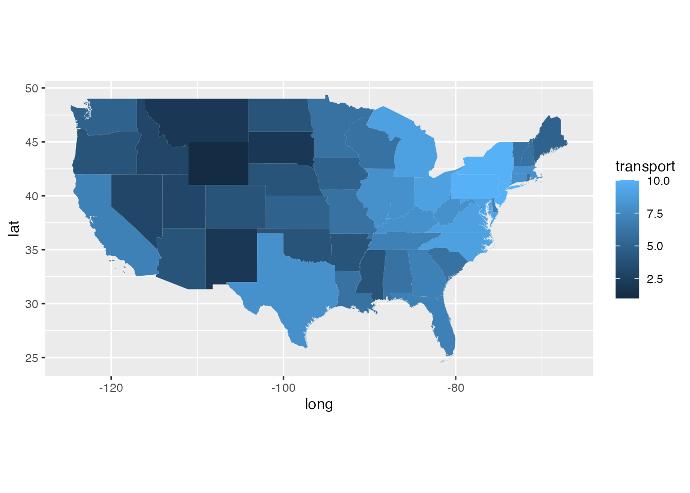
ggplot(states_gg[!states_gg$id %in% c("Alaska", "Hawaii"),]) +
  geom_polygon(aes(x = long, y = lat, group = group, fill = establishment)) +
  coord_quickmap()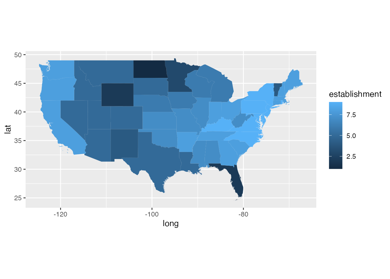
ggplot(states_gg[!states_gg$id %in% c("Alaska", "Hawaii"),]) +
  geom_polygon(aes(x = long, y = lat, group = group, fill = impact_wine)) +
  coord_quickmap()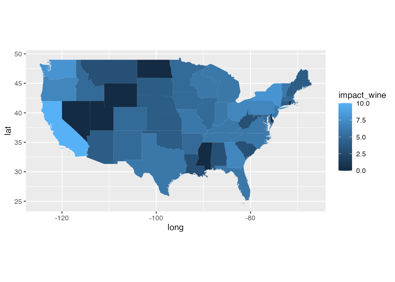
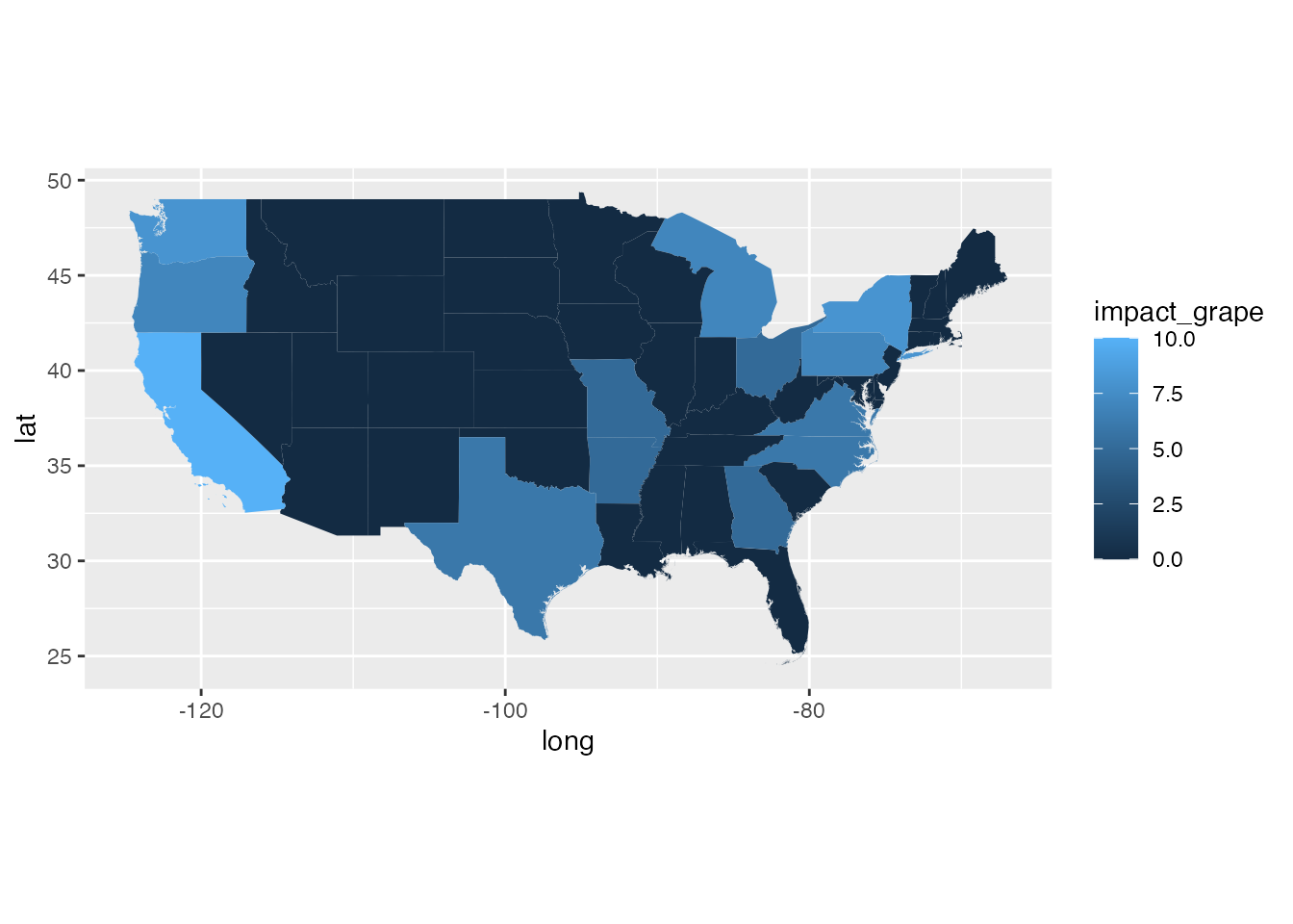
ggplot(states_gg[!states_gg$id %in% c("Alaska", "Hawaii"),]) +
  geom_polygon(aes(x = long, y = lat, group = group, fill = impact_grape)) +
  coord_quickmap()