Species Distribution Modeling • slfrsk

How to Build, Evaluate, and Save Species Distribution Models for Ailanthus altissima (TOH) and Lycorma delicatula (SLF)

This vignette is designed to demonstrate the workflow that lead to the creation of the three species distribution models (SDMs) used to assess the risk of SLF paninvasion. The description will not include actual running of some steps of this workflow, as some are unwieldy. Instead, information to ensure proper replication of those steps is provided. Notably, the MaxEnt runs are not conducted in this vignette, although the means to do so within R may be possible.

The scope of this vignette is as follows:

Reading and Visualization of Presence Data
Preparation of Spatial Data
Evaluation of Spatial Data Collinearity
Building and evaluating MaxEnt SDMs
Visualizing SDMs and Extracting Summary Statistics by Geopolitical Unit

Setup

We load the packages that are necessary to complete any analyses that allow us to demonstrate the workflow. Packages may include comments to clarify their purpose or the steps in which they are used.

library(slfrsk) #this package, has extract_enm()
library(tidyverse)  #data manipulation
library(here) #making directory pathways easier on different instances
library(ENMTools) #enviro collinearity analyses
library(patchwork) #easy combined plots
library(scales) #rescale the plots easily
library(rgdal) #load shapefiles
library(doParallel) #parallized extraction

1. Reading and Visualization of Presence Data

We built models of both SLF and TOH from presence records obtained from public databases (as seen in the “GBIF Records” vignette). As is standard practice, we checked all records for quality, removed duplicate and imprecise records, and obtained 8,022 TOH and 325 SLF unique and cleaned presence records.

#load data
data("slf_points")
data("toh_points")

#plot points on map: TOH
map_toh <- ggplot() +
  geom_polygon(data = map_data('world'), aes(x = long, y = lat, group = group), fill = "#FFFFFF", color = "black", lwd = 0.15) + #world map
  geom_point(data = toh_points, aes(x = x, y = y), color = "#0072b2", alpha = 0.10) +
  theme_bw() +
  labs(x = "", y = "") +
  theme(panel.grid.major = element_blank(),
        panel.grid.minor = element_blank(),
        #plot.background = element_rect(fill ="#f0f8ff"),
        panel.background = element_rect(fill = "#f0f8ff")) +  
  coord_quickmap(xlim = c(-164.5, 163.5), ylim = c(-55,85)) +
  ggtitle(label = "TOH Presence")

#plot points on map: SLF
map_slf <- ggplot() +
  geom_polygon(data = map_data('world'), aes(x = long, y = lat, group = group), fill = "#FFFFFF", color = "black", lwd = 0.15) + #world map
  geom_point(data = slf_points, aes(x = x, y = y), color = "#d55e00", alpha = 0.50) +
  theme_bw() +
  labs(x = "", y = "") +
  theme_bw() +
  theme(panel.grid.major = element_blank(),
        panel.grid.minor = element_blank(),
        #plot.background = element_rect(fill ="#f0f8ff"),
        panel.background = element_rect(fill = "#f0f8ff")) +
  coord_quickmap(xlim = c(-164.5, 163.5), ylim = c(-55,85)) +
  ggtitle(label = "SLF Presence")

#patchwork output of both maps
map_toh / map_slf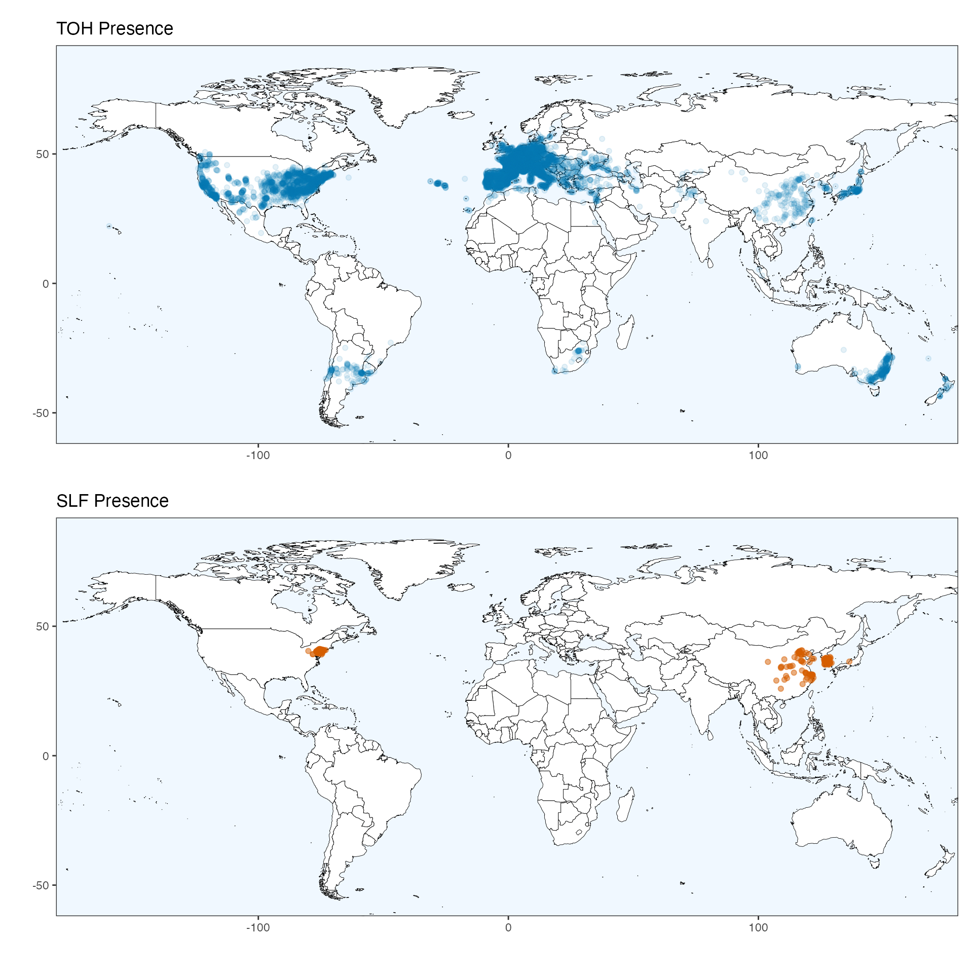


#ggsave((map_toh / map_slf), filename = file.path(here(), "slf_toh_presence.png"), height = 10, width = 10)

ggplot() +
  geom_polygon(data = map_data('world'), aes(x = long, y = lat, group = group), fill = "#FFFFFF", color = "black", lwd = 0.15) + #world map
geom_point(data = toh_points, aes(x = x, y = y), color = "#0072b2", alpha = 0.10) +
geom_point(data = slf_points, aes(x = x, y = y), color = "#d55e00", alpha = 0.50) +
  theme_bw() +
  labs(x = "", y = "") +
  theme(panel.grid.major = element_blank(),
        panel.grid.minor = element_blank(),
        #plot.background = element_rect(fill ="#f0f8ff"),
        panel.background = element_rect(fill = "#f0f8ff")) +
  #theme_bw() +
  coord_quickmap(xlim = c(-164.5, 163.5), ylim = c(-55,85))

2. Preparation of Spatial Data

To discern which environmental variables to use in the species distribution models (SDMs), we had to minimize collinearity among included covariates (A. Townsend Peterson et al. (2011)). To do so, we estimated pairwise correlation coefficients for 22 global raster covariates hypothesized to influence SLF and TOH distributions: the 20 WorldClim topographic and bioclimatic variables (Hijmans et al. (2005), Fick and Hijmans (2017)), forest height (Simard et al. (2011)), and access to cities (Weiss et al. (2018)).

To limit the raster data of covariates to the area of interest, we cropped their extent to \([-180, 180]\) for latitude and \([-60, 84]\) for longitude and ensured that the extent and resolutions matched one another by using one layer as a reference raster with raster::resample(method = "bilinear). This corrected any mismatching among cropped rasters of different sources (example code below).

if(FALSE){  #open no run if
  
#my path to the GoogleDrive shared directory
mypath <- "/Volumes/GoogleDrive/Shared drives/slfData/data/slfrsk/raw_env"
  
#ensure that extent is identical
#get file names
env.files <- list.files(file.path(mypath, "originals"), pattern = "[.]tif", full.names = T)
env.short <- list.files(file.path(mypath, "originals"), pattern = "[.]tif", full.names = F)

#change the labeling of the output layers
output.files <- env.short

#change weird BIOCLIM prefix
output.files <- gsub(pattern = "wc2.0_bio_30s", replacement = "global_bio", x = output.files)
#change weird ENVIREM prefix
output.files <- gsub(pattern = "current_30arcsec", replacement = "global_env", x = output.files)
#change weird ATC prefix
output.files <- gsub(pattern = "2015_accessibility_to_cities_v1.0", replacement = "global_atc", x = output.files)

#crop one of the BIOCLIM layers to set the bounding box and resolution to have files fixed
same.extent <- extent(-180, 180, -60, 84)
main_layer <- crop(raster(file.path(mypath,"originals", "wc2.0_bio_30s_01.tif")), y = same.extent, overwrite = F)

#reset extent stepwise
for(a in seq_along(env.files)){

  #ensure that the CRS is consistent
  rast.hold <- raster(env.files[a])
  crs(rast.hold) <- "+proj=longlat +datum=WGS84 +no_defs +ellps=WGS84 +towgs84=0,0,0"
  #resample to fit the extent/resolution of the reference BIOCLIM layer
  #use bilinear interpolation, since values are continuous
  rast.hold <- resample(x = rast.hold, y = main_layer, method = "bilinear")

  #write out the new resampled rasters!
  writeRaster(x = rast.hold, filename = file.path(mypath,"v1", output.files[a]), overwrite = T)
}

} #closes no run if

For tractability, we first downsized the resolution of these global covariate rasters with raster::aggregate(fact = 2, fun = mean, expand = TRUE, na.rm = TRUE) before assessing collinearity (see example code below). However, the full resolution covariates were used to build all models.

if(FALSE){  #open no run if
  
#my path to the GoogleDrive shared directory
mypath <- "/Volumes/GoogleDrive/Shared drives/slfData/data/slfrsk/raw_env"
  
#list the enviro layers to load sequentially
env.files <- list.files(path = file.path(mypath, "v1"), pattern = ".tif", full.names = T)
env.short <- list.files(path = file.path(mypath, "v1"), pattern = ".tif", full.names = F)

#downsampling by a factor of 2 (read 2 cells deep around a cell) and take the mean of the cells
for(a in seq_along(env.files)){
  holder <- raster(env.files[a])
  down_holder <- raster::aggregate(holder, fact = 2, fun = mean, expand = TRUE, na.rm = TRUE, filename =file.path(mypath, "v1_downsampled", env.short[a]), overwrite = T)
}

} #closes no run if

3. Evaluation of Spatial Data Collinearity

To evaluate the correlations among the covariates, we used ENMTools::raster.cor.matrix(method = "pearson"). Note that this code may still take quite some time to run. For brevity, we have included a version of the correlation matrix with the compendium for quick review (location: /data-raw/env_cor_v1_downsampled.csv).

if(FALSE){  #open no run if

#my path to the GoogleDrive shared directory
mypath <- "/Volumes/GoogleDrive/Shared drives/slfData/data/slfrsk/raw_env"

#load the downsampled layers and stack for raster.cor.matrix command

#list of layer paths
env.files <- list.files(path = file.path(mypath,"v1_downsampled"), pattern = ".tif", full.names = T)

#stack the downsized layers
env <- raster::stack(env.files)

#evaluate correlations for raster layers
#create a correlation matrix for picking model layers
env.corr <- ENMTools::raster.cor.matrix(env, method = "pearson")

#write out the correlations as a csv
write.csv(x = env.corr, file = file.path(here(),"data-raw", "env_cor_v1_downsampled.csv"), col.names = TRUE, row.names = TRUE)

} #closes no run if

To visualize the correlations between pairs of environmental covariates easily, we take the absolute value of all correlations and present the strength of relationships as a heatmap.

#re-read the correlation table in again
env.cor <- read.csv(file = file.path(here::here(),"data-raw", "env_cor_v1_downsampled.csv"), row.names = 1)

#here, we make cor's absolute values and make the data tidy to make it easier to plot in ggplot2
p_env_cor <- env.cor %>%
  abs(.) %>%
as_tibble() %>%
  mutate(covar = colnames(.)) %>%
  dplyr::select(covar, everything()) %>%
  pivot_longer(cols = -covar, names_to = "var") %>%
  dplyr::select(var, covar, everything()) %>%
ggplot() +
  geom_tile(aes(x = var, y = covar, fill = value)) +
  viridis::scale_fill_viridis(discrete = FALSE, direction = -1, limits = c(0,1), name = "abs(Correlation)") +
  guides(x =  guide_axis(angle = 90)) +
  labs(x = "", y = "")

p_env_cor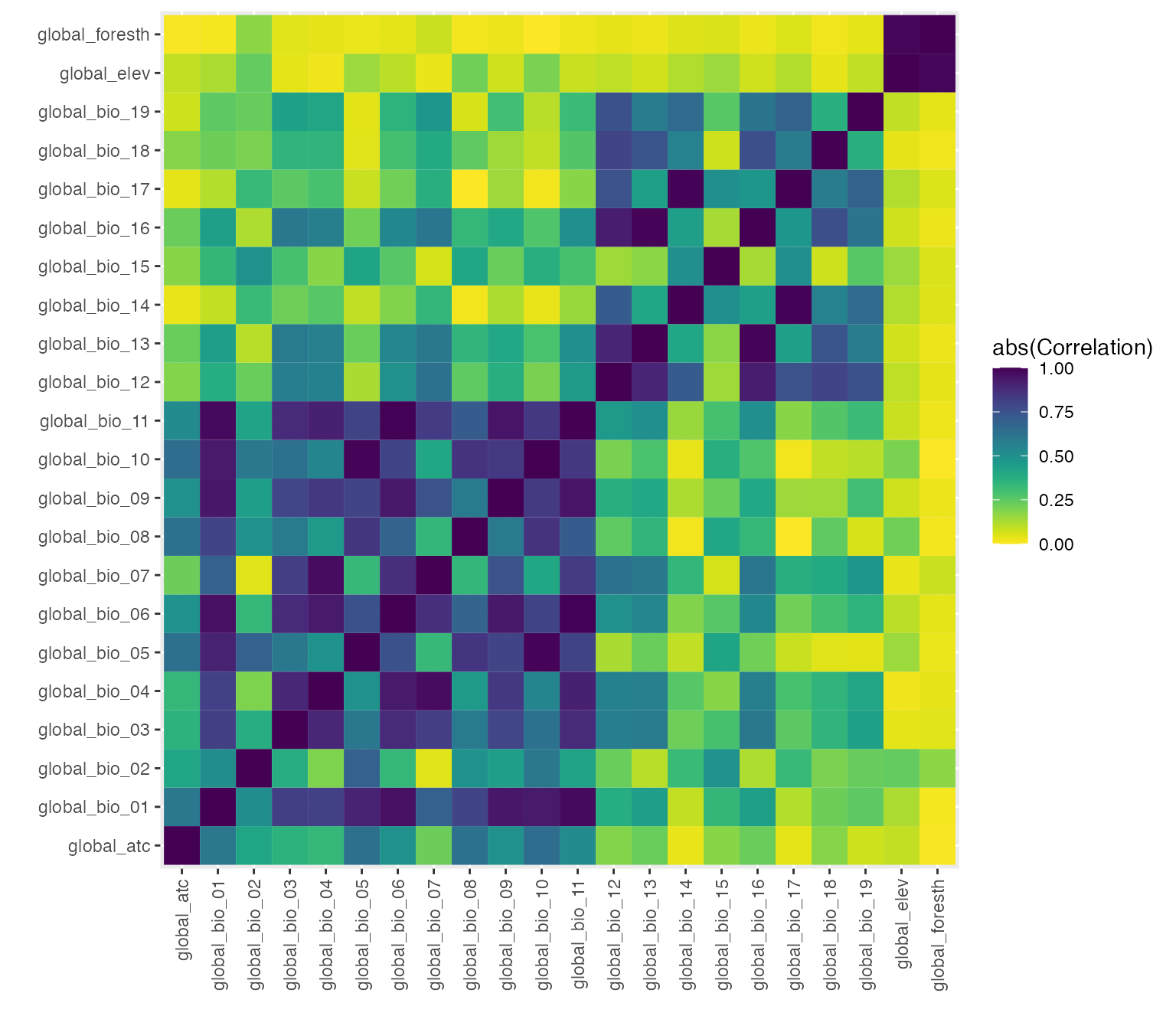


#ggsave(p_env_cor, filename = file.path(here(), "p_env_cor.png"), height = 10, width = 10)

With the correlations, we identified 6 of the 22 covariates that had minimal cross-correlations: annual mean temperature (BIO01), mean diurnal temperature range (BIO02), annual precipitation (BIO12), precipitation seasonality (BIO15), elevation (ELEV), and access to cities (ATC). These variables were then converted to ASCII files (.asc), as required by MaxEnt (example code below). We also set all NA values to -9999, which is the default value recognized as NA by MaxEnt.

Note that these .asc files are massive. It is not advisable to run this chunk unless you are certain that you have sufficient space to do so. It is for this reason (in part) that we do not provide this file type for all covariates.

if(FALSE){  #open no run if

#my path to the GoogleDrive shared directory
mypath <- "/Volumes/GoogleDrive/Shared drives/slfData/data/slfrsk/raw_env"

#get and set file names  
env.files <- list.files(path = file.path(mypath,"v1"), pattern = "[.]tif", full.names = T)
env.short <- list.files(path = file.path(mypath,"v1"), pattern = "[.]tif", full.names = F)
env.asc <- gsub(pattern = ".tif", replacement = ".asc", x = env.short)

#loop to convert and make sure to set NA values to -9999
for(a in seq_along(env.files)){
  file_to_asc <- raster(env.files[a])
  NAvalue(file_to_asc) <- -9999
  writeRaster(x = file_to_asc, filename = file.path(mypath, "v1_maxent", env.asc[a]), format = "ascii", overwrite = F)
}

  } #closes no run if

4. Building and evaluating MaxEnt SDMs

Focal Models

To further evaluate environmental covariates, we modeled each of them individually with SLF. To do this, we used MaxEnt (v3.4.1, available at https://biodiversityinformatics.amnh.org/open_source/maxent/) under default parameters, excluding the following changes (Phillips, Anderson, and Schapire (2006), Pearson et al. (2007)):

All feature types were made available but still set to Auto Features (Linear, Quadratic, Product, Threshold, and Hinge set to TRUE before setting Auto Features to TRUE)
Create response curves was set to TRUE
Do jackknife to measure variable importance was set to TRUE
Replicates set to 5 for SLF (this sets the number of k-fold crossvalidation replicates and determines the test proportion from k)
Apply threshold rule set to Minimum training presence
Threads set to the available number of processor threads available

After fitting individual models, we fit these 6 covariates combined to SLF and TOH presences, except that the number of Replicates = 10 for TOH, rather than Replicates = 5. The resultant two models are:

sdm_toh—a multivariate SDM of TOH
sdm_slf1—a multivariate SDM of SLF

A third model was created from sdm_toh suitability and SLF presence records, based on evidence supporting the strong affinity of SLF for TOH as a preferred host (Parra, Moylett, and Bulluck (2018), (urban_perspective:_2019?)):

sdm_slf2—a single variate SDM of SLF

Here, we report in a simple table the metrics used to evaluate the various models that were considered as well as the percent contribution of each variable to each model (where applicable). Model validation was conducted with k-fold cross-validation (k partitions discussed above) via evaluation of the receiver operating characteristic of the AUC and omission error (Fielding and Bell (1997), Phillips, Anderson, and Schapire (2006), Pearson et al. (2007), Anderson and Gonzalez (2011)).

For AUC, the fraction of true positives relative to type I error (positive background points) is compared at all possible thresholds for each model (Fielding and Bell (1997), Phillips, Anderson, and Schapire (2006)). The resultant plot’s area under the curve is assessed relative to a random model (\(AUC = 0.50\)), such that values close to \(1.00\) indicate strong model performance and those \(\leq 0.50\) suggest poor performance (Fielding and Bell (1997)). Given presence only data, measured AUC cannot reach \(1.00\), but model AUCs that approach \(1.00\) are considered to perform well (Wiley et al. (2003), Phillips, Anderson, and Schapire (2006)).

Given recent concerns with model evaluation with AUC (A. Townsend Peterson, Papeş, and Soberón (2008), Lobo, Jiménez-Valverde, and Real (2008), Jiménez‐Valverde (2012)), we confirmed model performance with average omission error, which measures the proportion of presence point(s) predicted with suitability less than the minimum training presence threshold (Pearson et al. (2007), Anderson and Gonzalez (2011)).

#read in summary table and view
data("models_summary")

#print results
knitr::kable(models_summary)

model	avg_test_auc	avg_omission_error	atc_contribution	bio01_contribution	bio02_contribution	bio12_contribution	bio15_contribution	elev_contribution
sdm_toh	0.7779	0.0003	61.03	36.74	0.06	1.08	0.81	0.28
sdm_slf1	0.9828	0.0064	57.16	22.97	1.95	11.63	5.96	0.32
sdm_slf2	0.9675	0.0032	NA	NA	NA	NA	NA	NA

The three models performed similarly, albeit with small differences across model performance metrics. Notably, the variables that contributed most the sdm_toh also contributed most to sdm_slf1, albeit at differing amounts. Thus, we created a consensus output map by averaging the three models as an ensemble.

To visualize the models and produce the ensemble model image, we first had to convert the mean model for each set of replicates (species_name_avg.asc) and convert it to a GeoTIFF (.tif), which is more easily visualized and stored (example code below).

if(FALSE){  #open no run if

#my path to the GoogleDrive shared directory
mypath <- "/Volumes/GoogleDrive/Shared drives/slfData/data/slfrsk/raw_env"

#read in file as ASCII raster
enm_data_slf <- raster(file.path(mypath, "maxent_models", "10_21_20_maxent_slf_full", "Lycorma_delicatula__White,_1845__avg.asc"))

#make sure CRS is WGS84
crs(enm_data_slf) <- "+proj=longlat +datum=WGS84 +no_defs +ellps=WGS84 +towgs84=0,0,0"

#write out as a geotiff
writeRaster(x = enm_data_slf, filename = file.path(mypath,"maxent_models", "slf.tif"), format = "GTiff")

  } #closes no run if

Ensemble Model

To create the ensemble model image, we averaged the three models (see code below). The resultant model image was used to extract summary statistics by geopolitical unit.

if(FALSE){  #open no run if

#my path to the GoogleDrive shared directory
mypath <- "/Volumes/GoogleDrive/Shared drives/slfData/data/slfrsk/raw_env"

#read in a geotiff version of the maxent suitability for all three models
toh <- raster(file.path(mypath,"maxent_models", "toh.tif"))
slf <- raster(file.path(mypath,"maxent_models", "slf.tif"))
slftoh <- raster(file.path(mypath,"maxent_models", "slftoh.tif"))

#stack the rasters
enm_data <- stack(c(toh, slf, slftoh))

#make mean raster
enm_ensemble <- mean(enm_data)

#write out the resulting file
writeRaster(x = enm_ensemble, filename = file.path(mypath, "maxent_models", "slftoh_ensemble_mean.tif", format = "GTiff")

  } #closes no run if

5. Visualizing SDMs and Extracting Summary Statistics by Geopolitical Unit

Visualization

To make visualization more tractable, we reduced the size of the SDMs by using raster::aggregate(fun = mean, expand = TRUE, na.rm = TRUE) (setting fact= to 4 for states and 10 for countries) to reduce the SDM raster resolution (more specific example code can be found in data-raw/downsample_raster_models.R for downsampling and data-raw/convert_data_rda.R for fortify()-ing rasters to plot rasters easily with ggplot2). We also clipped the SDMs to the continental US to produce the files used for separate states and countries visualization. The three models can be visualized below for the US and then the world:

USA Maps

#read in the data
data("slf_usa_df")
data("slftoh_usa_df")
data("toh_usa_df")

#plot just the states and suitability first
sdm_toh_usa <- ggplot() +
  geom_raster(data = toh_usa_df, aes(x = x, y = y, fill = rescale(value)), alpha=0.9, show.legend = F) +
  scale_fill_gradientn(limits= c(0,1), name = "Suitability", colors = rev(c("#e31a1c","#fd8d3c", "#fecc5c", "#FFFFFF"))) +
  geom_polygon(data = map_data('state'), aes(x = long, y = lat, group = group), fill = NA, color = "black", lwd = 0.10) +
  theme_bw() +
  labs(x = "", y = "") +
  theme(panel.grid.major = element_blank(),
        panel.grid.minor = element_blank(),
        panel.background = element_blank()) +
  coord_quickmap(xlim = c(-124.7628, -66.94889), ylim = c(24.52042, 49.3833)) +
  ggtitle(label = "sdm_toh USA")
sdm_slf1_usa <- ggplot() +
  geom_raster(data = slf_usa_df, aes(x = x, y = y, fill = rescale(value)), alpha=0.9, show.legend = F) +
  scale_fill_gradientn(limits= c(0,1), name = "Suitability", colors = rev(c("#e31a1c","#fd8d3c", "#fecc5c", "#FFFFFF"))) +
  geom_polygon(data = map_data('state'), aes(x = long, y = lat, group = group), fill = NA, color = "black", lwd = 0.10) +
  theme_bw() +
  labs(x = "", y = "") +
  theme(panel.grid.major = element_blank(),
        panel.grid.minor = element_blank(),
        panel.background = element_blank()) +
  coord_quickmap(xlim = c(-124.7628, -66.94889), ylim = c(24.52042, 49.3833)) +
  ggtitle(label = "sdm_slf1 USA")
sdm_slf2_usa <- ggplot() +
  geom_raster(data = slftoh_usa_df, aes(x = x, y = y, fill = rescale(value)), alpha=0.9, show.legend = T) +
  scale_fill_gradientn(limits= c(0,1), name = "Suitability", colors = rev(c("#e31a1c","#fd8d3c", "#fecc5c", "#FFFFFF"))) +
  geom_polygon(data = map_data('state'), aes(x = long, y = lat, group = group), fill = NA, color = "black", lwd = 0.10) +
  theme_bw() +
  labs(x = "", y = "") +
  theme(panel.grid.major = element_blank(),
        panel.grid.minor = element_blank(),
        panel.background = element_blank()) +
  coord_quickmap(xlim = c(-124.7628, -66.94889), ylim = c(24.52042, 49.3833)) +
  ggtitle(label = "sdm_slf2 USA")

#visualize together
sdm_toh_usa / sdm_slf1_usa / sdm_slf2_usa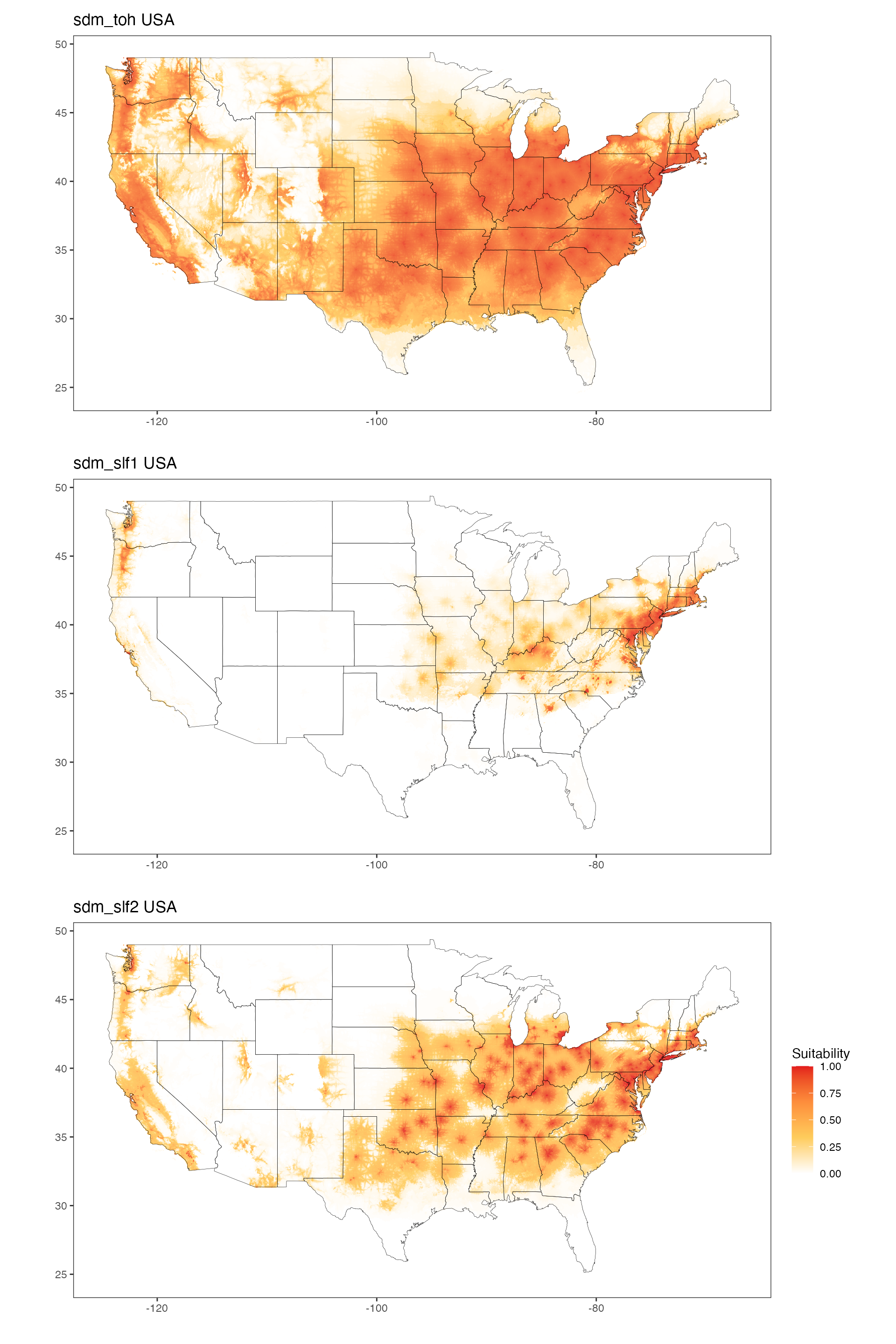


#ggsave(sdm_toh_usa, filename = file.path(here(), "sdm_toh_usa.png"), height = 5, width = 10)
#ggsave(sdm_slf1_usa, filename = file.path(here(), "sdm_slf1_usa.png"), height = 5, width = 10)
#ggsave(sdm_slf2_usa, filename = file.path(here(), "sdm_slf2_usa.png"), height = 5, width = 10)

World Maps

Please note that the images for countries are downsized considerably to ensure that the visualization data can be included with the package.

#read in the data
data("slf_df")
data("slftoh_df")
data("toh_df")

#plot just the states and suitability first
sdm_toh <- ggplot() +
  geom_raster(data = toh_df, aes(x = x, y = y, fill = rescale(value)), alpha=0.8, show.legend = F) +
  scale_fill_gradientn(limits= c(0,1), name = "Suitability", colors = rev(c("#e31a1c","#fd8d3c", "#fecc5c", "#FFFFFF"))) +
  geom_polygon(data = map_data('world'), aes(x = long, y = lat, group = group), fill = NA, color = "black", lwd = 0.15) +
  theme_bw() +
  labs(x = "", y = "") +
  theme(panel.grid.major = element_blank(),
        panel.grid.minor = element_blank(),
        panel.background = element_blank()) +
  coord_quickmap(xlim = c(-164.5, 163.5), ylim = c(-55,85)) +
  ggtitle(label = "sdm_toh")
sdm_slf1 <- ggplot() +
  geom_raster(data = slf_df, aes(x = x, y = y, fill = rescale(value)), alpha=0.8, show.legend = F) +
  scale_fill_gradientn(limits= c(0,1), name = "Suitability", colors = rev(c("#e31a1c","#fd8d3c", "#fecc5c", "#FFFFFF"))) +
  geom_polygon(data = map_data('world'), aes(x = long, y = lat, group = group), fill = NA, color = "black", lwd = 0.15) +
  theme_bw() +
  labs(x = "", y = "") +
  theme(panel.grid.major = element_blank(),
        panel.grid.minor = element_blank(),
        panel.background = element_blank()) +
  coord_quickmap(xlim = c(-164.5, 163.5), ylim = c(-55,85)) +
  ggtitle(label = "sdm_slf1")
sdm_slf2 <- ggplot() +
  geom_raster(data = slftoh_df, aes(x = x, y = y, fill = rescale(value)), alpha=0.8, show.legend = T) +
  scale_fill_gradientn(limits= c(0,1), name = "Suitability", colors = rev(c("#e31a1c","#fd8d3c", "#fecc5c", "#FFFFFF"))) +
  geom_polygon(data = map_data('world'), aes(x = long, y = lat, group = group), fill = NA, color = "black", lwd = 0.15) +
  theme_bw() +
  labs(x = "", y = "") +
  theme(panel.grid.major = element_blank(),
        panel.grid.minor = element_blank(),
        panel.background = element_blank()) +
  coord_quickmap(xlim = c(-164.5, 163.5), ylim = c(-55,85)) +
  ggtitle(label = "sdm_slf2")

#visualize together
sdm_toh / sdm_slf1 / sdm_slf2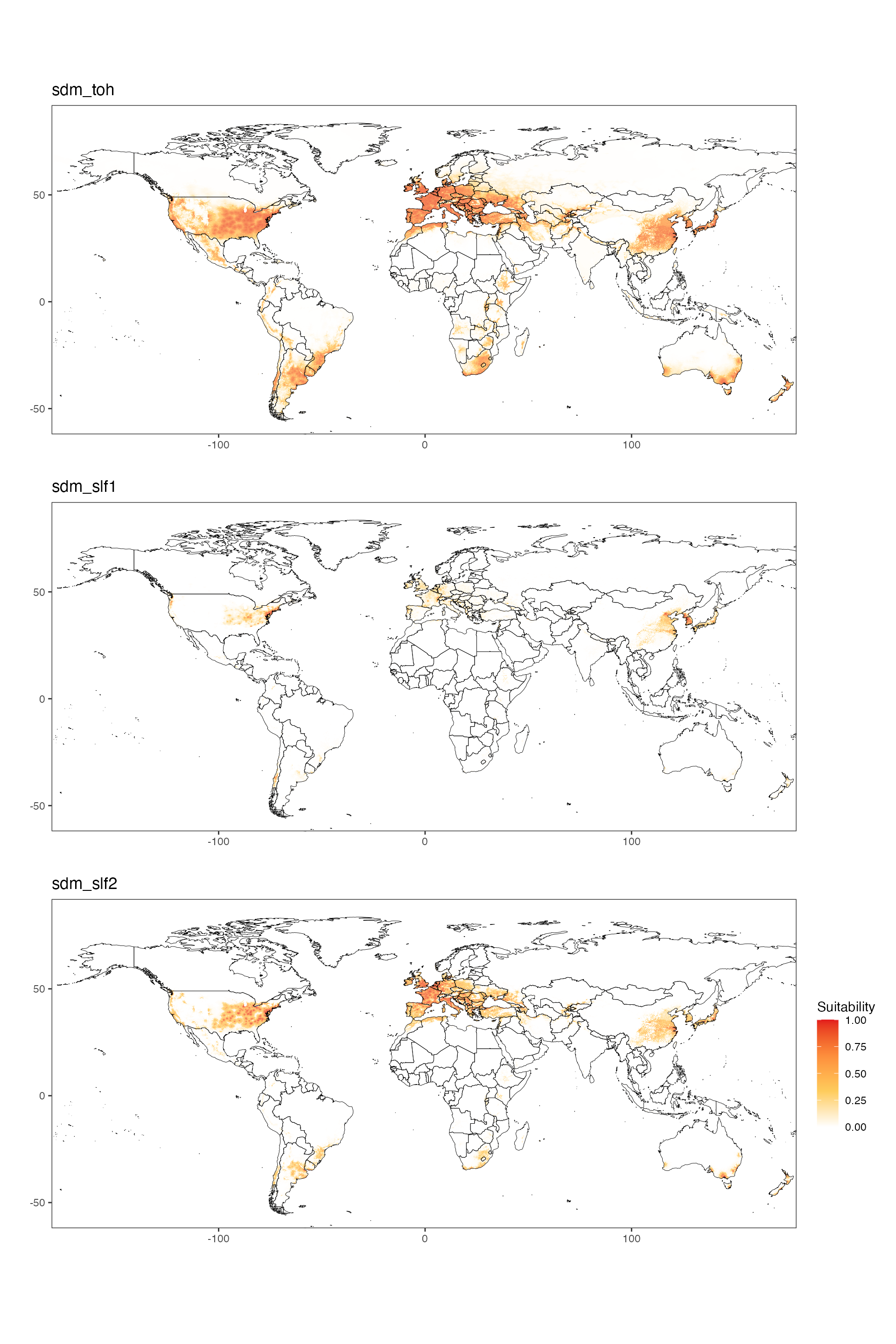


#ggsave(sdm_toh, filename = file.path(here(), "sdm_toh.png"), height = 5, width = 10)
#ggsave(sdm_slf1, filename = file.path(here(), "sdm_slf1.png"), height = 5, width = 10)
#ggsave(sdm_slf2, filename = file.path(here(), "sdm_slf2.png"), height = 5, width = 10)

Ensemble Maps

We can also visualize the ensemble images similarly (see the vignette-030-risk-maps for more detail versions). Note that these visualizations are also downsampled, albeit at fact=4 for both maps.

#read in data
data("suitability_usa_df")
data("suitability_countries_df")

en_usa <- ggplot() +
  geom_raster(data = suitability_usa_df, aes(x = x, y = y, fill = rescale(value)), alpha=0.9, show.legend = F) +
  scale_fill_gradientn(limits= c(0,1), name = "Suitability", colors = rev(c("#e31a1c","#fd8d3c", "#fecc5c", "#FFFFFF"))) +
  geom_polygon(data = map_data('state'), aes(x = long, y = lat, group = group), fill = NA, color = "black", lwd = 0.10) +
  theme_bw() +
  labs(x = "", y = "") +
  theme(panel.grid.major = element_blank(),
        panel.grid.minor = element_blank(),
        panel.background = element_blank()) +
  coord_quickmap(xlim = c(-124.7628, -66.94889), ylim = c(24.52042, 49.3833)) +
  ggtitle(label = "USA Ensemble")

en <- ggplot() +
  geom_raster(data = suitability_countries_df, aes(x = x, y = y, fill = rescale(value)), alpha=0.8, show.legend = T) +
  scale_fill_gradientn(limits= c(0,1), name = "Suitability", colors = rev(c("#e31a1c","#fd8d3c", "#fecc5c", "#FFFFFF"))) +
  geom_polygon(data = map_data('world'), aes(x = long, y = lat, group = group), fill = NA, color = "black", lwd = 0.15) +
  theme_bw() +
  labs(x = "", y = "") +
  theme(panel.grid.major = element_blank(),
        panel.grid.minor = element_blank(),
        panel.background = element_blank()) +
  coord_quickmap(xlim = c(-164.5, 163.5), ylim = c(-55,85)) +
  ggtitle(label = "Ensemble")

#visualize together
en_usa / en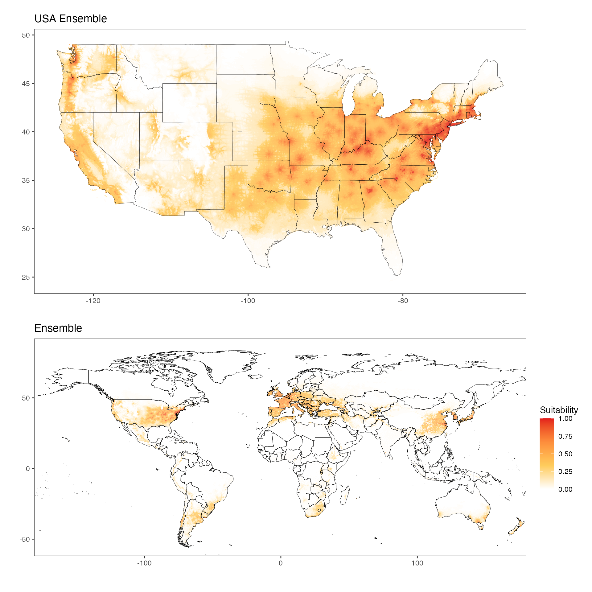


#ggsave(en_usa, filename = file.path(here(), "en_usa.png"), height = 5, width = 10)
#ggsave(en, filename = file.path(here(), "en.png"), height = 5, width = 10)

Extraction of Summary Statistics

With the three original and ensemble SDMs, we extracted summary statistics by geopolitical unit to later use for evaluation of suitability. To do this, we use a custom function (slfrsk::extract_enm()) that uses a reference shapefile (we use a saved copy of GADM data v3.6 for the world and US—both can be obtained online, https://gadm.org/data.html) to isolate the portion of the raster contained within each geopolitical unit and calculate the following summary statistics for suitability values:

mean
standard deviation
minimum
maximum
quantiles at the following probabilities:
- 0.25
- 0.50 (median)
- 0.75
- 0.90

Here, we demonstrate how we used this function to extract the summary statistics for each state and country used as our measure of establishment potential. Note that we do not use the save.plots argument or save the output. We also use the .tif versions of full-scale models for these extractions, due to their smaller size. We show code that works for the ensemble but also include commented-out code to run for an individual model and calculate rsa.

if(FALSE){  #open no run if

#my path to the GoogleDrive shared directory
mypath <- "/Volumes/GoogleDrive/Shared drives/slfData/data/slfrsk/raw_env"

#shapefile of world by countries
world <- readOGR(file.path(mypath, "geo_shapefiles", "gadm36_levels_shp", "gadm36_0.shp"), verbose = F, p4s = '+proj=longlat +datum=WGS84 +no_defs +ellps=WGS84 +towgs84=0,0,0')
#shapefile of US states (same sourcce as usa data)
states <- readOGR(dsn = file.path(mypath, "geo_shapefiles", "gadm36_USA_shp", "gadm36_USA_1.shp"), verbose = F, p4s = '+proj=longlat +datum=WGS84 +no_defs +ellps=WGS84 +towgs84=0,0,0')

#load data to test
  #ensemble model
enm_ensemble <- raster(file.path(mypath, "maxent_models", "slftoh_ensemble_mean.tif"))

#example of running the function
#extract the states
states_extracts_ensemble <- extract_enm(enm = enm_ensemble, geoshape = states, id0 = "NAME_1", id = as.character(states$NAME_1))
#optional save the summary data
write_csv(path = file.path(here(),"data-raw", "extract_states_slftoh_ensemble_mean.csv"), x = states_extracts_ensemble[[1]], col_names = T)

#countries version
countries_extracts_ensemble <- extract_enm(enm = enm_ensemble, geoshape = world, id0 = "NAME_0", id = as.character(world$NAME_0))

write_csv(path = file.path(here(),"data-raw", "extract_countries_slftoh_ensemble_mean.csv"), x = countries_extracts_ensemble[[1]], col_names = T)

#parallelized version
countries_extracts_ensemble2 <- extract_enm2(enm = enm_ensemble, geoshape = world, id0 = "NAME_0", id = as.character(world$NAME_0), multipar = TRUE, ncores = 4)
#write out
write_csv(path = file.path(here(),"data-raw", "extract_countries_slftoh_ensemble_mean2.csv"), x = countries_extracts_ensemble2, col_names = T)


#example with s3
#the threshold if desired:   enm_slftoh$`Minimum training presence Cloglog threshold`[nrow(enm_slftoh)]

#enm_data_slftoh <- raster(file.path(mypath, "maxent_models/11_07_18_maxent_slf+toh_+atc-bio02/lycorma_delicatula_avg.asc"))
#enm_data_slftoh <- raster(file.path(mypath, "maxent_models/slftoh.tif"))
#enm_slftoh <- read_csv(file.path(mypath, "maxent_models/11_07_18_maxent_slf+toh_+atc-bio02/maxentResults.csv"))
#state_extracts_slftoh <- extract_enm(enm = enm_data_slftoh, geoshape = states, id0 = "NAME_1", id = as.character(states$NAME_1), th = enm_slftoh$`Minimum training presence Cloglog threshold`[nrow(enm_slftoh)])

  } #closes no run if

Ultimately, the saved versions of these extracted suitabilities are saved in /data-raw and then can be handled by the script in the same directory, convert_data-rda.R, to be converted into .rda file(s), which are stored in /data and used by the other vignettes (with few, if any, exceptions that use a shared GoogleDrive). Any exceptions should be reproducible with the relevant raw starting files (INSERT HERE).

References

Anderson, Robert P., and Israel Gonzalez. 2011. “Species-Specific Tuning Increases Robustness to Sampling Bias in Models of Species Distributions: An Implementation with Maxent.” Ecological Modelling 222 (15): 2796–2811. https://doi.org/10.1016/j.ecolmodel.2011.04.011.

Fick, Stephen E., and Robert J. Hijmans. 2017. “WorldClim 2: New 1-Km Spatial Resolution Climate Surfaces for Global Land Areas.” International Journal of Climatology 37 (12): 4302–15. https://doi.org/10.1002/joc.5086.

Fielding, Alan H., and John F. Bell. 1997. “A Review of Methods for the Assessment of Prediction Errors in Conservation Presence/Absence Models.” Environmental Conservation 24 (1): 38–49. https://doi.org/10.1017/S0376892997000088.

Hijmans, Robert J., Susan E. Cameron, Juan L. Parra, Peter G. Jones, and Andy Jarvis. 2005. “Very High Resolution Interpolated Climate Surfaces for Global Land Areas.” International Journal of Climatology 25 (15): 1965–78. https://doi.org/10.1002/joc.1276.

Jiménez‐Valverde, Alberto. 2012. “Insights into the Area Under the Receiver Operating Characteristic Curve (AUC) as a Discrimination Measure in Species Distribution Modelling.” Global Ecology and Biogeography 21 (4): 498–507. https://doi.org/10.1111/j.1466-8238.2011.00683.x.

Lobo, Jorge M., Alberto Jiménez-Valverde, and Raimundo Real. 2008. “AUC: A Misleading Measure of the Performance of Predictive Distribution Models.” Global Ecology and Biogeography 17 (2): 145–51. https://doi.org/10.1111/j.1466-8238.2007.00358.x.

Parra, Greg, Heather Moylett, and Russ Bulluck. 2018. “USDA-APHIS-PPQ-CPHST Technical Working Group Summary Report Spotted Lanternfly, Lycorma Delicatula (White, 1845).”

Pearson, Richard G., Christopher J. Raxworthy, Miguel Nakamura, and A. Townsend Peterson. 2007. “Predicting Species Distributions from Small Numbers of Occurrence Records: A Test Case Using Cryptic Geckos in Madagascar.” Journal of Biogeography 34 (1): 102–17. https://doi.org/10.1111/j.1365-2699.2006.01594.x.

Peterson, A Townsend, Jorge Soberón, Richard G Pearson, Robert P Anderson, Enrique Martínez-Meyer, Miguel Nakamura, and Miguel B Araújo. 2011. Ecological Niches and Geographic Distributions. Princeton University Press.

Peterson, A. Townsend, Monica Papeş, and Jorge Soberón. 2008. “Rethinking Receiver Operating Characteristic Analysis Applications in Ecological Niche Modeling.” Ecological Modelling 213 (1): 63–72. https://doi.org/10.1016/j.ecolmodel.2007.11.008.

Phillips, Steven J., Robert P. Anderson, and Robert E. Schapire. 2006. “Maximum Entropy Modeling of Species Geographic Distributions.” Ecological Modelling 190 (3-4): 231–59. https://doi.org/10.1016/j.ecolmodel.2005.03.026.

Simard, Marc, Naiara Pinto, Joshua B. Fisher, and Alessandro Baccini. 2011. “Mapping Forest Canopy Height Globally with Spaceborne Lidar.” Journal of Geophysical Research: Biogeosciences 116 (G4). https://doi.org/10.1029/2011JG001708.

Weiss, D. J., A. Nelson, H. S. Gibson, W. Temperley, S. Peedell, A. Lieber, M. Hancher, et al. 2018. “A Global Map of Travel Time to Cities to Assess Inequalities in Accessibility in 2015.” Nature 553 (7688): 333–36. https://doi.org/10.1038/nature25181.

Wiley, E O, Kristina M McNyset, A Townsend Peterson, C Richard Robins, and Aimee M Stewart. 2003. “Niche Modeling and Geographic Range Predictions in the Marine Environment Using a Machine-Learning Algorithm” 16 (3): 8. https://doi.org/https://doi.org/10.5670/oceanog.2003.42.